云计算 阅读材料 16 Case Studies - NoSQL Databases

In this module, we discuss a few popular NoSQL data stores: Apache HBase, MongoDB, Apache Cassandra and Amazon's DynamoDB.

---

As you may recall from earlier in this unit, the NoSQL movement in databases was primarily motivated by the big-data challenges of scale and performance. As an example, Google's BigTable was created to handle the massive amounts of information that the company deals with every day. For example, Google's Web index grew from 26 million pages in 1998 to over 1 trillion unique URLS in 2008. Processing such large amounts of data using a relational model becomes cumbersome if not impossible. In addition, big-data problems, such as Web analytics, do not require the specific constraints and ACID guarantees that are provided by relational database management systems (RDBMSs) but instead can benefit from a flexible data model that relaxes some of the consistency guarantees for performance and scalability.

The adage "use the right tool for the job" is appropriate because NoSQL databases are not always the right fit for every kind of problem. NoSQL databases typically excel at managing large amounts of data that may not be fully structured (in a strict schema). Certain types of data can be represented better in one of the NoSQL database forms, such as a key-value, document, or graph database, rather than in the relational database model. Some NoSQL databases, such as Apache Cassandra, even support a fully nested data model, which allows for complex data structures to be present as a value in the database.

NoSQL databases are not a good fit in situations in which the data is fairly well structured and defined and may not exceed a few gigabytes or terabytes in size. Most NoSQL databases rely on a large number of machines organized as a cluster to process data in parallel. As an example, if HBase or Cassandra is run on a single node, the performance of either may not match that of MySQL or any other RDMBS product.

A good example of a nonrelational database that is a good fit for NoSQL databases is a webtable (Figure 3.38). A webtable is a data structure that holds results of a Web crawl. A Web crawl is the process of visiting a list of Web pages and following the links in them in order to catalog and index the information that is contained in a website.

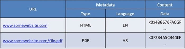
Each unique URL in a Web crawl can be stored as a row in a webtable, with the URL being the unique identifying characteristic of that row, which makes the URL the key. The columns of the webtable can store the binary content and metadata of the URL. As the webtable is parsed, new columns can be added with semantic information derived from the HTML content, such as the links of other pages in the URL object, and any other information. The webtable can also act as the database back end for a Web archive service, such as an Internet archive, and hence clients can directly retrieve objects using the URL as the key.

Creating a webtable for a few URLs may be a simple task that can be handled by a traditional RDBMSs, but when billions of websites need to be crawled and their information has to be stored in a table that may be accessed by hundreds of thousands of clients simultaneously, then the data store is best maintained on a large cluster using a NoSQL solution.

Apache HBase

Apache HBase is an open-source version of Google's BigTable distributed storage system and is supported by the Apache Software Foundation. BigTable is a distributed, scalable, high-performance, versioned database. BigTable's infrastructure is designed to store billions of rows and columns of data in loosely defined tables, such as the webtable described earlier. Video 4.16 contains an overview of HBase.

Video 4.16: HBase

Just as traditional RDBMSs are designed to run on top of a local file system, HBase is designed to work on top of the Hadoop Distributed File System (HDFS). As described earlier, HDFS is a distributed file system that stores files as replicated blocks across multiple servers. HDFS lends a scalable and reliable file system back end to HBase.

HBase Data Model

Applications store data organized as rows and columns in a table, which loosely resemble tables in an RDBMS. To illustrate, we organize the webtable example as an HBase table in Figure 4.39.

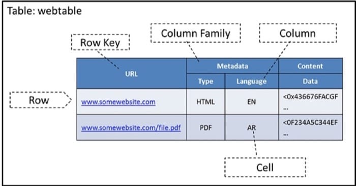
A row in HBase is referenced using a row key, which can be considered to be the primary key of the table in an RDBMS. The primary key of the table has to be unique and hence reference one and only one row. Unlike in RDBMSs (which require primary keys to be of certain types), row keys are raw byte arrays, so theoretically, anything from strings to binary representations of long integers, floats, or even entire data structures that have been serialized (converted to a byte array form) can serve as a row key. HBase automatically sorts table rows by row key when it stores them. By default, this sort is byte ordered.

Columns in HBase have a column name, which can be used to refer to a column. Columns can be further grouped into column families. All column family members have a common prefix, so, in the webtable example, the columns Metadata:Type andMetadata:Language are both members of the Metadata column family, whereasContent:Data belongs to the Content family. By default, the colon character (:) delimits the column prefix from the family member. The column family prefix must be composed of printable characters. The qualifying tail can be made of any arbitrary bytes.

HBase differs from an RDBMS because the columns do not need to be typed; they are simply interpreted as raw byte strings. This interpretation enables HBase to store any kind of data in the table but also prevents it from being able to automatically validate data values when they are loaded into the table.

Although a table's column families must be defined up front when creating the table, the family members can be added on demand. HBase stores all of the column's family members together on the underlying file system. Thus, HBase is a columnar database.

Table cells, the intersection of row and column coordinates, are versioned (i.e., HBase stores multiple versions [default being 3] of the values stored in its tables). The version of a table cell value is timestamped and automatically assigned by HBase at the time of cell insertion or update. Thus, the tuple {row,column,version} fully describes a unique value stored in an HBase table.

HBase Operations

HBase has four primary operations on the data model: Get, Put, Scan, and Delete.

A Get operation returns all of the cells for a specified row, which are pointed to by a row key. A Put operation can either add new rows to the table when used with a new key or update a row if the key already exists. Scan is an operation that iterates over multiple rows based on some condition, such as a row key value or a column attribute. A Delete operation removes a row from a table. Get and Scan operations always return data in sorted order. Data are first sorted by row key, then by column family, then by family members, and finally by timestamp (so the latest values appear first).

By default, Get, Scan, and Delete operations on an HBase table are performed on data that have the latest version. A Put operation always creates a new version of the data that are put into HBase. By default, Delete operations delete an entire row but can also be used to delete specific versions of data in a row. Each operation can be targeted to an explicit version number as well.

HBase Architecture

HBase is organized as a cluster of HBase nodes. These nodes are of two types: a master node and one or more slave nodes (called RegionServers; Figure 4.40). HBase uses Apache ZooKeeper as a distribution coordination service for the entire HBase cluster. For example, it handles master selection (choosing one of the nodes to be the master node), the lookup for the -ROOT- catalog table (explained shortly), and node registration (when new regionservers are added). The master node that is chosen by ZooKeeper handles such functions as region allocation, failover, and load balancing.

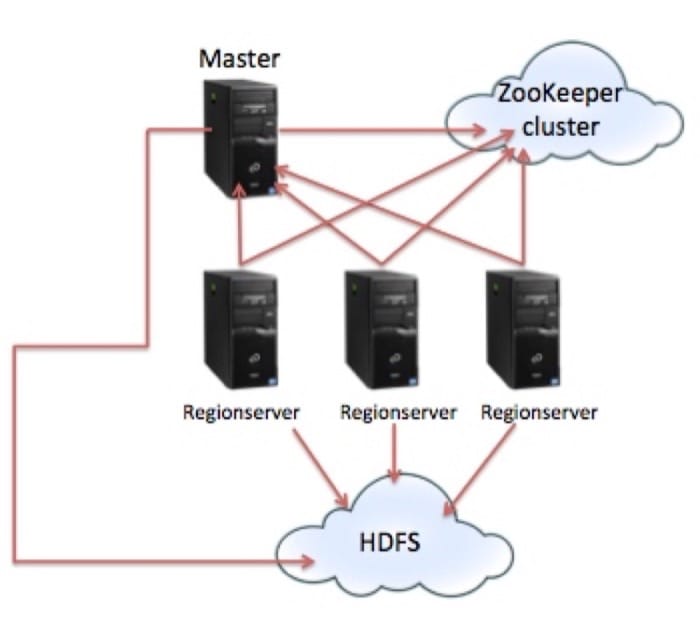
As with most databases, HBase is able to persist data using an underlying file system. HBase is designed to use HDFS in the back end but also supports various kinds of file systems, including a local file system and even Amazon S3. Typically, every regionserver in HBase is also an HDFS DataNode (an HDFS fileserver), but this is not mandatory in HBase.

Data Partitioning

HBase is designed to scale tables to a large number of rows and columns (in the millions), with the size of each table running into terabytes or petabytes. At this scale, it is impossible to host the data on a single node. To distribute data stored in HBase across the nodes in a cluster, HBase automatically partitions (shards) tables intoregions, which are groups of consecutive rows in a table (Figure 4.41).

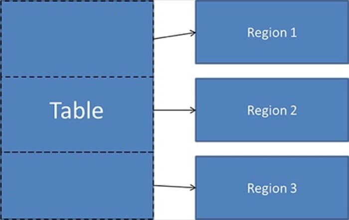
Each region is defined by the base row (inclusive) and the last row (exclusive) as well as a region identifier (a randomly generated number). Tables are initially stored in a single region, but as the size of the table reaches a certain threshold, HBase automatically generates a new region by splitting the data into two nearly equal regions. This process continues as the tables continue to get larger.

Client Access

HBase clients can connect to HBase to perform the operations on HBase tables, as described in the data model. However, the clients must locate the appropriate node in the HBase cluster that stores the region of the table that needs to be accessed. To keep track of all of the regions and their location in the HBase cluster, HBase has twocatalog tables, called -ROOT- and .META. in HBase parlance. These tables are also treated as HBase tables and can be stored anywhere in the HBase cluster for fault-tolerance purposes. The -ROOT- table is always self-contained in a single region, while the .META. table may be split into multiple regions. A client first connects to the cluster to learn the location of the -ROOT- table (via ZooKeeper) and then queries the -ROOT-table to elicit the location of the .META. table. The .META. table then returns the location of the actual row requested by the client. Once the regionserver is resolved by the client, the client directly interacts with that regionserver and performs the required row operations.

The client also caches the -ROOT- and .META. tables after the first access so that consecutive client operations do not require additional lookups to these tables. The client will continue to use its cached copy of the catalog tables until it encounters a fault, which typically means that the catalog tables have been updated after the location of a table region has moved. The client updates its cached copy of the catalog tables and continues with the operation.

Write Operations

A regionserver handles write operations in the following manner: the write operation is appended to a commit log on HDFS (which is triple replicated by default), after which the write operation is added to an in-memory cache. When this in-memory cache of the regionserver becomes full, its content is flushed to the file system.

Because the commit log is stored on HDFS, it remains available through a regionserver crash. When the master notices that a regionserver is no longer reachable, it retrieves the commit log and splits the changes across regions. Each regionserver gets a portion of the commit log and replays the edits to bring the file system to its prefailure, consistent state.

Read Operations

For read operations, HBase always consults the in-memory cache of a region. If sufficient versions of the data are found to satisfy the query, the data are returned. Otherwise, the flushed files are consulted in order from newest to oldest to find the required data or until there are no more flush files to consult. A background process periodically compacts the flush files once their number reaches a certain threshold by combining many flush files into one. During compaction, any versions of cells beyond a user-configured threshold (default value is 3) of deleted rows are cleared out.

ACID Properties in HBase

HBase, like many NoSQL databases, is not fully ACID compliant by design. HBase does guarantee ACID compliancy for a row but not on operations that span rows. ACID properties in HBase are as follows:

• Atomicity: HBase offers atomicity for operations that update individual rows. Any Put operation will either succeed in its entirety or fail. Operations that update multiple rows can either succeed or fail on individual rows, and HBase will return the status per row.
• Consistency: HBase offers a consistent view of a database for Get operations on a single row. The data returned will be data that existed at some point in the table's history. In addition, any edits done to the table will be seen in the order they were completed. However, the HBase Scan operation is not strictly consistent. For example, if a Scan operation runs simultaneously with an operation that updates one or more rows that are part of the scan, the Scan operation may return rows that have been updated or that have not been updated. It is important to note that a row is always updated in its entirety and never partially updated.
• Isolation: Operations on a row are performed in order and hence are strictly isolated from each other. However, as explained in the previous bullet, scans are not isolated from other operations on individual rows.
• Durability: HBase guarantees durability on all data that are visible. Any data returned from a read will always be on a disk in some form.

HBase Use Cases

HBase offers multiple interfaces with which to work. The Java interface to HBase can be used in a MapReduce job. In addition, HBase has a REST interface, which can be used to retrieve data stored in HBase through HTTP service calls.

HBase shares the same use cases as Google's Big Table. HBase is a distributed data store that can store billions of rows and columns.

HBase is best suited for big-data storage, which requires fast access to multiple rows at a time for aggregations, such as summing or averaging. The model also allows for flexibility of adding columns to the database at any time. The versioning property of HBase is also useful to store information that changes over time, but previous versions of the data are also useful. In the webtable example, multiple versions of a Web page can be stored for comparison.

HBase does not support the join operation, where data from two or more tables are combined on a common column to create another table. If your application is dependent on joins, then HBase may not be the right choice. In addition, HBase's relaxed consistency model places additional burdens on the application developer, for example, to verify the results of scans.

References

1. Apache Software Foundation (2014). The Apache HBase™ Reference Guide. O'Reilly Media/Yahoo Press. http://hbase.apache.org/book/book.html.

MongoDB

MongoDB is a document-oriented database. MongoDB eschews the relational model in favor of a "schema-less" model, which is designed to be more flexible and mimics the way data is modeled in modern object-oriented programming languages. MongoDB is also designed to be scalable from the ground up, it can automatically split up data among multiple servers and balance load across servers in a cluster. MongoDB also allows for complex queries such as those that involve MapReduce-style aggregations and geo-spatial queries, making MongoDB popular as a data store for mapping-related applications. Video 4.42 covers MongoDB

Video 4.42: MongoDB

MongoDB Data Model

A document is the basic unit of data for MongoDB, roughly equivalent to a row in a relational database management system. A document is an ordered set of keys and their associated values. An example of a document is illustrated below:

{
    item: "ABC1",
    details: {
    model: "14Q3",
    manufacturer: "XYZ Company"
    },
    stock: [ { size: "S", qty: 25 }, { size: "M", qty: 50 } ],
    category: "clothing"
}

MongoDB stores documents in groups known as a collection. MongoDB does not impose any restriction on the documents that are part of a collection. They can contain any number or type of keys and do not have to be related. The only restriction is that every document in a collection has a key called _id, which should have a unique value for every document in a collection. MongoDB can automatically generate the _id key for each document inserted into a collection.

A collection is identified by a UTF-8 string known as the name of the collection. Many developers choose to group collections together using a naming convention, like using the . character to denote two types of blog collections: blog.posts and blog.authors. This is purely for organization, and MongoDB treats them as separate, unrelated collections.

Finally, a group of collections make a MongoDB database. Just like collections, a MongoDB database is identified by a UTF-8 string name.

MongoDB supports a rich array of data types, including 32/64 bit integers, 64-bit floats, boolean values, dates, strings, regexes, javascript code, arrays and more. Documents can also be nested, i.e. a document can contain other documents within it, making MongoDB's data model fully nested.

Internally, documents are stored in MongoDB using a format called BSON (Binary JSON). The size of an individual document in MongoDB is restricted to 4MB.

Operations in MongoDB

The main operations in MongoDB to manipulated data are as follows: insert, removeand updates. MongoDB allows batch inserts, which lets an application insert multiple documents in a single request. The only restriction in MongoDB is the message size, which is 16MB. MongoDB also allows for a special kind of operation, known as anupsert. This operation will update an existing document or will insert a new document if it does not exist.

Data is queried in MongoDB using the find command. Using the find command with a set of conditions can be used to return documents which match a set of conditions. A subtle limitation in MongoDB is that the conditions used in the find command must be a constant value specified in the query itself. This means that you cannot write a query in MongoDB that finds documents in which a certain value matches another value from the collection.

Apart from simple queries, MongoDB provides a set of aggregation tools that can be applied on the set of resulting documents in a query. Aggregations range from simple counts to MapReduce functions to further distill and analyze the data returned from a query.

As with most database systems, MongoDB allows for the creation of indices on specific keys to be created for a collection. This can be used to reduce the time taken to execute certain types of queries. A salient feature of MongoDB is the ability to create indices on geospatial data keys, such as latitude and longitude. MongoDB can handle range queries on geo-spatial data efficiently.

MongoDB also allows administrators to ask the system to explain queries, similar to the capabilities afforded by popular RDBMSes. This allows administrators to analyze and optimize query execution in MongoDB.

MongoDB Architecture

MongoDB manages collections and documents as files on a local file system. If an index is created on a particular key, then MongoDB uses a B-Tree structure to store the index information. MongoDB essentially works on these files on disk in a memory-mapped fashion, leaving it to the OS and file system to manage the in-memory buffer for the files containing the data.

For small installations, MongoDB is deployed as as a single-node system. In order to scale MongoDB to multiple nodes, MongoDB support two scale-out modes:replication and sharding. In replication, multiple copies of the same data are maintained over multiple servers, allowing for MongoDB to tolerate node failures in case a node goes down. A set of mongodb nodes that has the same data is known as areplica set. One node in a replica-set is known as the primary, the remaining nodes are known as secondaries. By default, only the primary node responds to requests from clients for both reads and writes. The primary node sends out messages to update the replicas whenever there is an operation that writes data. In this mode, MongoDB guarantees strict consistency as all requests for data are processed only by the primary node.

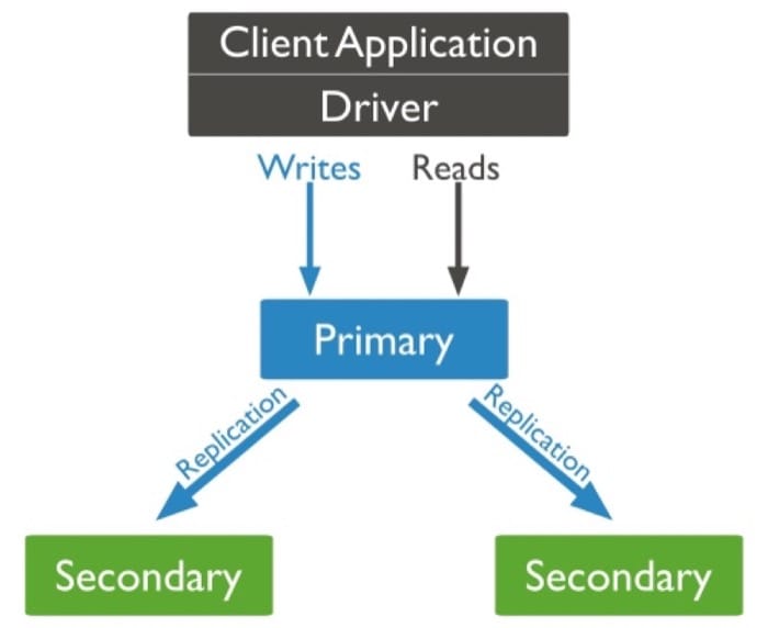
A MongoDB replica-set is designed for automatic failover. If a node fails to respond for more than 10 seconds, it is presumed to be dead and the remaining nodes vote on which node should be the new primary node.

In order to distribute data, MongoDB allows for data to be sharded across multiple nodes. Each shard is an independent database, and collectively, the shards make up a single logical database. The architecture of a sharded MongoDB cluster is illustrated below:

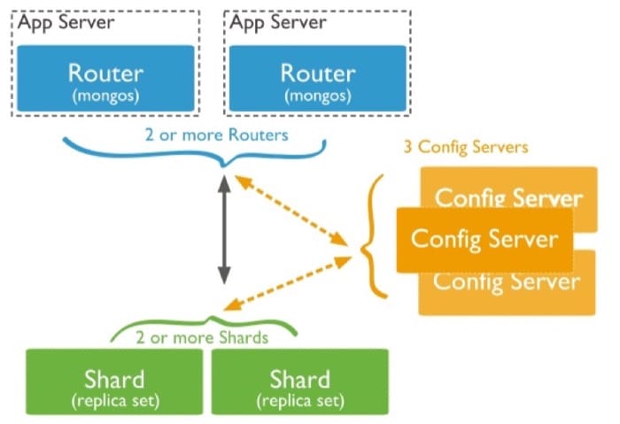
Shards store the data. To provide high availability and data consistency, in a production sharded cluster, each shard is a replica set.

Query Routers interface with client applications and direct operations to the appropriate shard or shards. The query router processes and targets operations to shards and then returns results to the clients. A sharded cluster can contain more than one query router to divide the client request load. A client sends requests to one query router. Most sharded clusters have many query routers.

Config servers store the cluster’s metadata. This data contains a mapping of the cluster’s data set to the shards. The query router uses this metadata to target operations to specific shards.

Data is distributed across multiple nodes using a specific key known as the shard key. MongoDB divides the shard key values into chunks and distributes the chunks evenly across the nodes in the cluster. The shard keys can either be hash-based or range based. In hash-based sharding the hash-value of a shard key is used to assign a document to a specific chunk. In range-based sharding, each chunk is assigned to a specific range of values of the shard key, and documents can then be assigned to a specific chunk.

MongoDB allows administrators to direct the balancing policy using tag aware sharding. Administrators create and associate tags with ranges of the shard key, and then assign those tags to the shards. Then, the balancer migrates tagged data to the appropriate shards and ensures that the cluster always enforces the distribution of data that the tags describe.

MongoDB Use Cases

MongoDB can be used to meet specific challenges for certain types of applications:

Large, rapidly evolving data set: MongoDB supports large amounts of data and has a very flexible schema-less design. For applications that evolve rapidly and require ever-changing schema, MongoDB may be a good choice.

Location-based data: MongoDB is unique in its ability to store and index geo-spatial data in an efficient manner. For this reason, MongoDB is used quite extensively for applications that use geo-spatial or map data. (Examples include booking applications, location-based services, etc)

Applications with a high write load: MongoDB has built-in support for bulk inserts and supports a high-insert rate, while having relaxed transaction safety when compared to RDBMSes.

High availability in an unreliable environment: MongoDB's architecture allows for near-instant, automatic recovery from the failure of a Node when replication is configured. This is especially useful in unreliable environments.

Apache Cassandra

Apache Cassandra is a fully distributed, structured key-value storage system. Cassandra marries the best aspects of both BigTable [1] and Amazon's Dynamo. [4]Cassandra uses the data model of BigTable and the implementation architecture of Dynamo. Video 4.18 covers Cassandra.

Video 4.18: Cassandra

Cassandra Data Model

Cassandra implements the data model of BigTable (which is similar to HBase's data model, as discussed on the previous page), with slightly different terminology.

A table in Cassandra is referred to as a column family (not to be confused with HBase's column family, which is a group of associated columns in a table); see Figure 4.45(a). A record (or row ) is treated as a key-value pair, with the key being an identifying characteristic of the record. The value is also considered to be a set of key-value pairs, where each key is the name of each column, and each value is the value in the column (Figure 4.45(b)).

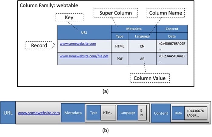
Like BigTable and HBase, Cassandra also allows for nested columns, which are known as super columns. Super columns in Cassandra are implemented as nested key-value pairs, where the super column name is the key, and the value is a sequence of key-value pairs that correspond to each column name and value.

Cassandra allows for data to be stored in the key or value parts of each key-value pair. Values can be stored in column or super column names, if required. Typical operations in Cassandra involve storing and retrieving individual rows using the key as well as updates to parts of a row. The data model in Cassandra is hence similar to BigTable and HBase and is fairly flexible to allow various types of data to be stored. The big difference between HBase's and Cassandra's data models is that Cassandra does not have built-in support for versioning like HBase.

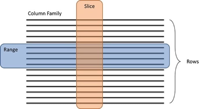
Cassandra supports data operations similar to HBase, with a few exceptions. Typical operations in Cassandra are expressed as Gets, Inserts, and Deletes. Operations can be performed on a single row or a set of rows (called a range). In addition, operations can be performed on a set of columns of a database (called a slice), as illustrated in Figure 4.46.

Cassandra Architecture

As a distributed data store, Cassandra is designed to run on a cluster of nodes, similar to HBase. However, unlike HBase, Cassandra follows a decentralized architecture(i.e., there is no master-slave architecture, and every node in Cassandra has the same role), which means Cassandra is designed without a single point of failure (SPOF). Although HBase is designed to be failure resilient, it relies on the Hadoop Distributed File System (HDFS) for persistent storage, where the NameNode is a SPOF. Cassandra does not require an underlying distributed file system (DFS); the nodes in a Cassandra cluster simply use the local storage on each node. Coordination between cluster nodes in Cassandra is handled in a peer-to-peer fashion.

Data Distribution in Cassandra

Client requests to read or write data in Cassandra can be serviced by any node in the cluster. As rows are inserted in a Cassandra column family, Cassandra automatically distributes these rows among the different nodes in a cluster. However, the technique used to distribute the rows is vastly different from how they are distributed in HBase. Data in Cassandra are distributed among the nodes based on the hash value of the key of a row using a strategy called consistent hashing.

Consistent Hashing

Cassandra automatically distributes rows among the various nodes in the cluster using the hash value of the key of each row. In the default case, Cassandra uses a Message Digest 5 (MD5) hashing algorithm on the key of each row, generating hashes that are 128 bits long. The hash value of a key determines where the row is stored in the cluster. In order to distribute rows across the nodes in a Cassandra cluster evenly, each node in the cluster is given a unique token. A token is a range of hash values that is assigned to each node. By default, node tokens are a range of values from 0 to 2127, which are equally divided by the number of nodes in the cluster. The collection of all of the nodes of the cluster is collectively referred to as a token ring, with the nodes arranged in order. Every node in the token ring is aware of the other nodes in the token ring and the range of hash values for which they are responsible. An example is illustrated in Figure 4.47.

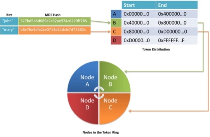
In the example, the key john has an MD5 hash value that starts with hex value 5. The node that fits this range in the token ring is B (it accepts hash values ranging from 0x4to 0x8). Thus, the row with the key john is stored on node B. Similarly, mary is stored on node C because its hash value starts with B, and node C is responsible for all values from 0x8 to 0xD.

It is important to note that the Cassandra administrator can manually partition the token space among the nodes, assigning specific ranges of the hash space to any node. Thus, consistent hashing provides a natural load-balancing mechanism for a Cassandra cluster. We now explore how the consistent hashing scheme provides replication and fault tolerance to a Cassandra cluster.

Replication

Although the data distribution policy in Cassandra evenly distributes the data among the nodes in the cluster, if one of them fails, the rows that are stored on that node can be potentially lost. To provide redundancy against node failures, Cassandra replicates rows across multiple nodes, as defined by the replication factor (which is 1 by default). Cassandra offers both a rack-aware and a rack-unaware strategy for replica placements. The first replica is always placed based on the hashing technique described before.

Assume that the replication factor specified is N. The first replica is always placed using the consistent hashing technique described before. In the rack-aware strategy, the second replica is always placed at another data center (if the Cassandra cluster spans data centers) or to another rack from the first replica. The remaining replicas are placed on nodes that are on the same rack as the first, in the order of the nodes in the token ring. In the rack-unaware strategy, replicas are simply placed in order along the next N-1 nodes in the token ring.

Nodes can be added to a Cassandra cluster at any time, which is handled in two ways. Either the administrator manually reassigns tokens for the new incoming node, or Cassandra automatically finds the node with the most data and divides its token in half, giving one half of the hash space to the new incoming node. The new node will not immediately accept requests because it must first learn the topology of the ring and accept data that it may also be responsible for. After it has done so, it can join the ring as a full member and begin accepting requests. Cassandra then reshuffles the data among the nodes in the cluster.

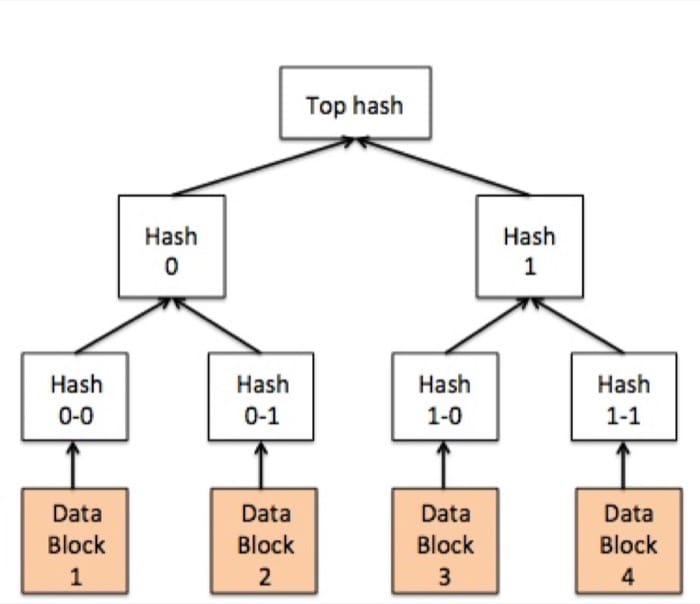
The process of keeping replicas up to date in Cassandra is called antientropy. Antientropy in Cassandra is achieved using Merkle trees. [2] A Merkle tree (Figure 4.48) is a hash tree in which the leaves are hashes of the values of individual keys. Parent nodes higher in the tree are hashes of their respective children. The principal advantage of Merkle trees is that each branch of the tree can be checked independently without having to scan the entire branch. Cassandra periodically computes the Merkle trees for each column family and exchanges it among replica members to quickly compute differences in the tables so that they can be synchronized. Compared to other techniques in Cassandra, antientropy is an expensive operation that is not performed often. Cassandra also has techniques to perform instantaneous repairs to replicas during reads (called a read repair, which is described later).

Data Operations in Cassandra

Write Operations

When a write operation is sent to a Cassandra node, it is first written to the commit log (on the local file system) for that node. The commit log is a type of journal that ensures that the write operation can be recovered in case of any crashes. The write is then forwarded to the memtable, which is a memory-resident data structure (a form of cache). The memtable allows the data to be memory resident, allowing future operations to read the values directly from memory and improving performance. When the memtable size reaches a certain threshold, Cassandra flushes it to the disk in a file called the SSTable, and then a new memtable is created. The flush operation is nonblocking, and hence other operations on that Cassandra node do not have to wait for the flush to complete before proceeding.

Delete Operations

Delete operations are treated as update operations that place a tombstone (a delete marker) on the value to be removed, meaning that data is not purged from Cassandra immediately but is marked for deletion (this is also called a soft delete). Values are not deleted until a garbage collection grace seconds value is reached, and by default, this value is 864,000 seconds (approximately 10 days). After the expiry of the garbage collection threshold, the tombstones are marked as expired.

Compaction Operations

As the Cassandra instance is running, it may have collected multiple SSTables (through many flushes). An operation called compaction is performed periodically to merge the data from multiple SSTables. In the compaction operation, the keys are merged, the columns are merged, expired Tombstones are deleted, and a new index is created.

Read Operations

To read data from a Cassandra cluster, a client connects to any node in the cluster and, based on the consistency level specified by the client, the read request is forwarded to a number of nodes in the client. This read operation is blocked until the required consistency level is met. If some of the nodes respond with an out-of-date value, then the most recent value is returned to the client. Cassandra then performs a read-repair operation. This operation is in addition to the periodic antientropy operation discussed previously. The read-repair operation brings the replicas up to date. The read repair is performed according to the consistency level specified during the read, which is explained next.

Tunable Consistency

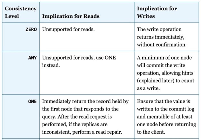
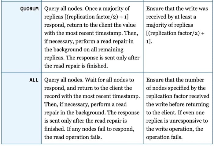
Unlike other NoSQL database systems, Cassandra has a tunable consistency model. Applications that make requests to Cassandra for read and write operations can specify a consistency level required from Cassandra for that operation. Thus, the application can specify the consistency level required for each operation. Cassandra supports up to five consistency levels, as outlined in the following table.

Failure Detection in Cassandra

Accrual Failure Detection

With no centralized master to keep track of the nodes in the cluster, Cassandra uses a special gossip protocol to communicate in all nodes in the token ring. In Cassandra, failures are expressed as a probability using an accrual failure detection (AFD) [3]algorithm, which can be summarized as follows.

Every second or so, each node in the Cassandra token ring contacts another random member in the ring to inquire about its status. This communication happens using a handshake protocol similar to a TCP handshake. In case the node cannot be contacted, a failure suspicion is raised. Therefore, the failure monitoring system outputs a continuous level of suspicion regarding how confident it is that a node has failed, which is desirable because it can account for fluctuations in the network environment. For example, just because one connection gets caught up, it does not necessarily mean that the whole node is dead. So a suspicion offers a more fluid and proactive indication of the weaker or stronger possibility of failure based on interpretation, as opposed to a simple binary assessment, such as dead or alive in heartbeat mechanisms.

Hinted Handoff

When data needs to be written to a location that is no longer reachable (due to some kind of failure), Cassandra implements a strategy called hinted handoff. The node that originally received the write request detects that the target node (where the write is to be performed) is down. The node then creates a hint, which is a reminder of that write operation. Informally, the hint is the equivalent of a person taking a message for someone who is not present. The hint would be that "I have this write information that is intended for node X. I am going to hold on to this write, and when I notice node Xhas come back online, I will send the write request to node X." This strategy allows Cassandra to be available for writes. Under the ANY write consistency model, a hinted handoff counts as a successful write.

ACID Properties of Cassandra

Unlike other database systems, Cassandra's ACID properties are entirely configurable on a per-operation basis. Cassandra's ACID properties are as follows:

• Atomicity: Cassandra guarantees atomicity in a column family for all the columns of a row, if the write has persisted on at least one commit log.
• Consistency: Using the ALL or QUORUM consistency model for reads and writes, Cassandra is considered to be strongly consistent, but at the expense of availability (as reads and writes may fail). Using the weaker consistency models (e.g., ZERO, ANY, ONE) can improve performance (by reducing response time for clients), but at the expense of consistency. More formally, the consistency of Cassandra can be expressed in the following formula. If W is the write replica count,R is the read replica count, and N is the replication factor, then if W + R > N, the system is strongly consistent. In other words, this formula means that a combination of the read and write operations must access all of the replicas of a particular row for the operation to be strongly consistent. As an example, consider the state when W = 1 (for the ONE consistency level) and R = N (for the ALL consistency level). In this scenario, the system is considered to be strongly consistent. Similarly, if W = N and R = 1, then the system is strongly consistent. If we were to consider a QUORUM state with Q defined as N/2 + 1, and if W = R = Q (i.e., both reads and writes are done in QUORUM mode), then the system is considered to be consistent.
• Isolation: Since version 1.1, Cassandra can guarantee isolation of a write operation only for a particular row.
• Durability: Under the ALL, ONE, and QUORUM models, writes are guaranteed to be durable (they are written to the commit log). Under the ZERO and ANY models, the writes may not be durable because there is no guarantee that the writes were written to the commit log of any node.

Cassandra Use Cases

Cassandra is a unique data storage system with useful features, such as tunable consistency, high availability, and scalability. Cassandra is best deployed with a large number of servers, which allow users to take full advantage of these features.

Cassandra is also among the most powerful for its write performance, which is in part due to its architecture and tunable consistency model. Cassandra was primarily developed for applications in the social network space, where writes are frequent and read operations are less predictable.

Another feature that is useful in Cassandra is that it has out-of-the-box support for replicating across multiple data centers. The fault-tolerance mechanism is more dynamic in nature (compared to HBase/Hadoop) and will not mistake long latencies as failures. The schema-free data model is also good for evolving applications, where application changes may occur frequently.

The Cassandra project wiki has many use-case examples as well.

References

1. Chang, Fay, et al. (2008). "BigTable: A distributed storage system for structured data." ACM Transactions on Computer Systems (TOCS). Volume 26. Number 2.
2. Merkle, R. (1988). "A digital signature based on a conventional encryption function." Proceedings of CRYPTO (pp. 369–378). Springer-Verlag.
3. Hayashibara, Naohiro, et al. (2004). ""The φ accrual failure detector." Reliable Distributed Systems, 2004. Proceedings of the 23rd IEEE International Symposium on Reliable Distributed Systems.." IEEE.
4. DeCandia, Giuseppe, et al. (2007). ""Dynamo: Amazon's highly available key-value store." ACM SIGOPS Operating Systems Review. Vol. 41. No. 6." ACM.

Amazon's DynamoDB

DynamoDB is a proprietary, highly available NoSQL data store offered by Amazon Web Services. DynamoDB has evolved from Dynamo, a distributed key-value storage system first described by Amazon in [1] . Dynamo shares some of the properties of databases as well as distributed hash tables (DHTs) and is designed using several techniques in distributed systems, including consistent hashing, quorum, and antientropy.

DynamoDB Data Model

Information in DynamoDB is stored in Tables. A table consists of multiple items, each of which has one or more attributes. DynamoDB has a flexible schema, and items can have any number of attributes. The only restriction in DynamoDB is that the size of an item must not exceed 400KB (This includes the sum of the lengths of individual attributes names and values for a single item). An example of an item in DynamoDB is given below:

{                                        
   Title = "Book 101 Title"
   ISBN = "111-1111111111"
   Authors = "Author 1"
   Price = -2
   Dimensions = "8.5 x 11.0 x 0.5"
   PageCount = 500
   InPublication = true
   ProductCategory = "Book" 
} 

When a table is created in DynamoDB, one attribute must be designated as theprimary key of the table, and is used to identify every item in the table. The attribute must appear in every item in a DynamoDB table. Primary keys can be of two types: they can either be a Hash Type primary key, which consists of a single attribute as the key, a Hash and Range Type primary key, which consists of two attributes. In the hash and range type primary key, the first attribute is a hash index, while the second attribute is a range attribute.

DynamoDB supports attributes that can be scalar (such as number, string, binary, boolean or null values), multi-valued (as a string, number or binary set of values), or can be a document type (such as a list or map).

Operations in DynamoDB

DynamoDB provides operations to create, update and delete tables. Once a table is created users can set a performance level for the table (designated as provisioned throughput). This enables Amazon to configure the DynamoDB backend to be able to maintain a guaranteed performance level, measured as a number of requests/second that the table will handle.

DynamoDB allows users to add, update or delete items from a table. Operations that interact with a single item in DynamoDB are known as queries. DynamoDB also supports conditional updates, where an update to a table can happen based on a user-specified condition.

Operations that interact with multiple items at a time are known as scan. A scan will effectively read every single item in a DynamoDB table. DynamoDB has a 1MB limit on the amount of data returned by any single operation, including scans. As you can expect, scans can be slow in DynamoDB, especially when done on large tables.

DynamoDB Architecture

Amazon's DynamoDB is based on the Dynamo architecture, which was described in [1] . Amazon made changes to the architecture since, but the basic principles remain more or less the same. Dynamo uses many of the techniques discussed in the section on Cassandra above, including consistent hashing, replication, hinted hand-off, anti-entropy using merkle trees and more. Dynamo was among the first distributed systems to use a combination of all these techniques in a single system.

Consistency in DynamoDB

Data stored in DynamoDB tables are replicated across 3 Amazon data centers to ensure that data is not lost in the event of a data-center wide failure. DynamoDB gives users the option to specify the consistency of read operation. By default, all reads aseventually consistent and may not reflect the results of a recently completed write. If the application requires strong consistency, that can be specified when making the read request to DynamoDB; this results in a performance hit as multiple replicas may have to consulted before the result of a read can be sent back to the client, but all prior writes that were successfully completed will be reflected in the read operation.

DynamoDB Use Cases

DynamoDB can be used to meet specific challenges for certain types of applications:

Latency-sensitive applications: DynamoDB is engineered to provide extremely low latency, especially for read workloads.

Applications that require fast scalability and predictable performance: DynamoDB as a service is extremely easy to scale up as demand increases. AWS provides monitoring systems to inform application developers about the number of requests being served by a table. Based on this information, developers can request additional provisioned capacity from DynamoDB to handle higher loads. This makes DynamoDB one of the easiest services to scale out as demand increases.

Applications with a simple data model: DynamoDB's data model is extremely simplified and basically only allows for inserts and updates to data items index with a key. DynamoDB does not support complex queries such as joins and is slow on operations such as aggregations, which require scans of the entire table. DynamoDB is more suited for applications with more transactional workloads than analytical workloads.

References

1. DeCandia, Giuseppe, et al. (2007). ""Dynamo: Amazon's highly available key-value store." ACM SIGOPS Operating Systems Review. Vol. 41. No. 6." ACM.

Summary

• Apache HBase is an open-source version of Google's BigTable distributed storage system. Both systems are distributed, scalable, high-performance, versioned databases.
• HBase organizes data into tables, with each row of a table being indexed by a key, and data are stored in columns. Multiple columns can be grouped together into column families.
• HBase columns do not need to be typed; columns can be added on demand. HBase stores data on a disk columnwise, making it a columnar database.
• Data stored in HBase rows are versioned; by default, operations apply to the newest version of the data.
• HBase supports the Get, Put, Scan, and Delete operations.
• HBase is organized as a cluster of nodes; one node is designated the master, and the others are known as regionservers. ZooKeeper is used to manage the cluster. HDFS is typically used to store data in HBase.
• Data in a table are partitioned into regions and assigned individual regionservers; the HBase master keeps a record of the region assignments.
• HBase is not fully ACID compliant, particularly with operations that span rows. In such cases, subsequent requests for data from HBase can return stale data.
• HBase is best suited for big-data storage and supports fast access to multiple rows for aggregations. Multiple interfaces allow for connectivity to MapReduce and to Web applications.
• HBase does not support joins, and its consistency model must be considered while designing applications.
• MongoDB is a document store that stores doucuments in collections.
• MongoDB stores data internally using the Binary JSON (BSON) format.
• MongoDB can be scaled to multiple clusters using replication and sharding.
• MongoDB is popular for applications that require scale-out, have the need for fast, bulk writes, as well as data that needs to have geo-spatial indices.
• Cassandra is a fully distributed, structured key-value storage system, which uses multiple design aspects of BigTable and Dynamo.
• A table in Cassandra is known as a column family, with each record indexed by a key and consisting of columns; multiple columns can be grouped together into a super column.
• A row in Cassandra is returned as a sequence of nested key-value pairs.
• Typical operations in Cassandra include Gets, Inserts, and Deletes. They can be performed on individual rows, on groups of rows (a range), and on a group of columns (a slice).
• Cassandra runs on a cluster of nodes using decentralized, peer-to-peer architecture. Cassandra uses the local storage on each node to store data.
• Cassandra nodes are arranged into a token ring, and Cassandra automatically distributes rows among the various nodes in the cluster using the hash value of the key of each row through consistent hashing. Every node is aware of all other nodes in the token ring and automatically forwards client requests to the correct node.
• Cassandra replicates rows across nodes on the basis of a user-defined replication factor.
• Every operation in Cassandra is performed with a user-defined consistency level. The consistency level provides a tunable tradeoff of consistency versus performance for every operation.
• Specialized algorithms in Cassandra are utilized to handle failure detection; Cassandra nodes can temporarily keep track of write requests to offline nodes and forward them when the node comes back online (hinted handoff).
• Cassandra's ACID properties are configurable on a per-operation basis.
• Cassandra is popular because of its feature set, and its tunable consistency model provides a great deal of flexibility in designing applications.
• DynamoDB is a managed NoSQL service provided by AWS.
• DynamoDB's data model allows for a key to be designated as the primary, no other schema is required.
• DynamoDB is a good choice for applications that require a low-latency key-value store.