云计算 阅读材料 21 Distributed Analytics Engines for the Cloud - GraphLab

Machine-learning and data-mining (MLDM) problems are growing exponentially in scale today. Interest in analytics engines that can execute MLDM algorithms efficiently on distributed systems, such as clouds, is increasing correspondingly.

---

Designing, implementing, and testing distributed MLDM applications can be challenging because they usually require experts who know how to address synchronization, deadlocks, communication, scheduling, distributed-state management, and fault-tolerance concerns effectively. Many recent advances in MLDM algorithmic designs have focused on modeling such algorithms as graphs.

Expressing Data and Computation using a Graph Abstraction

As a motivating example, lets take a look at a few examples of data modelled as graphs and how computation can be expressed in this model. Mathematically, a graph is modelled as a set: G={V,E}, where V is a set of vertices vi and E is a set of edges ei. Furthermore, every edge ei in G represents an edge between exactly two vertices {vi,vj}∈V . There are many types of graphs; they can be undirected which means e={vi,vj}={vj,vi}∀e∈E (i.e. all edges are equivalent and bidirectional), or directed, where the edges are distinct and not equal. Graphs can also be weighted if an additional parameter, known as the weight wi exists ∀e∈E . Furthermore, vertices may also be weighted, and as we will see, this comes in handy in different applications. Typical graph computations include the calculation of the shortest path between two points, partitioning the graph into subgraphs based on some optimization metric (minimum number of edges cut, or maximum flow between the graphs), the calculation of maximum degree (the vertex with the most number of edges), and so on.

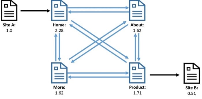
Figure 5.42 illustrates an example of the WebGraph. The vertices denote web pages and the edges denote links between web pages. The canonical example of computation performed on a webgraph is PageRank, which calculates the importance of a webpage, based on the pages that are linked to it. Recall the detailed description of PageRank we covered in the previous module. Similarly a social network graph illustrated in Figure 5.43 shows people represented as vertices and edges representing a relationship such as "is a friend", or "follows". Interesting computations here include calculation of the most popular people (calculating the vertices with the most number of edges), or finding strongly knit communities of people who all know each other (triangle counting).

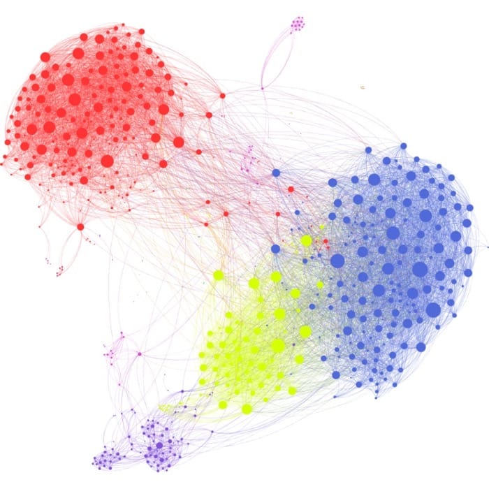
As you can imagine, some of the problems mentioned above are growing in scale and complexity. One of the largest publicly available webgraphs consists of 1.7 billion web pages and 64 billion hyperlinks, and is widely believed to be a much smaller than the data handled by production systems of web services companies such as Google and Microsoft. It would be impossible to encapsulate all this data into the memory of a single computer, but we still need efficient systems that can handle the processing of such large-scale data.

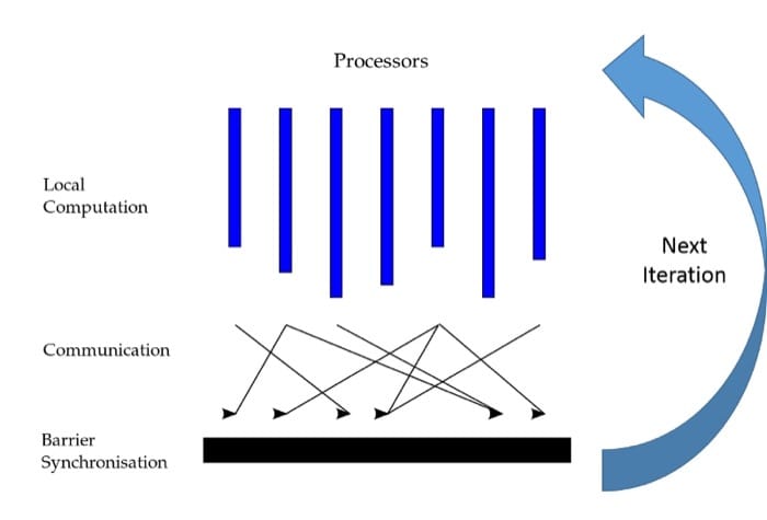
An example of a system designed to process large graphs in a distributed manner is Google's Pregel. Pregel performs computations on Graphs in an iterative, lock-step manner (also known as the Bulk-Synchronous Parallel or BSP approach). A Pregel program runs in a series of globally-synchronized iterations, which can result in some computation performed in the context of each vertex in a graph (Figure 5.44). The vertices can then exchange messages with their neighbours, typically this is done to update state or other variables. Pregel then runs the next iteration once all the vertices have completed processing the current execution. Messages exchanged between machines in iteration i are delivered in iteration i+1. The program will run subsequent iterations until either a convergence condition is met or it completed N iterations, where N is a user defined number of maximum iterations to be executed.

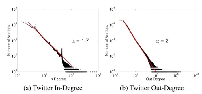
Although Pregel offers a promising option as a distributed, graph-parallel analytics engine it suffers from a major deficiency: Pregel runs computation synchronously, which can impact performance as the runtime of each iteration is always dictated by the last thread to complete execution. One can also imagine the implications if a graph is unbalanced in terms of the degree of vertices. This is in fact the case with a large number of graphs of interest to big data analytics. Social graphs, for example, show a power-law distribution, wherein a small number of vertices, have a large number of edges. An example of this phenomenon is the Twitter followers graph (Figure 5.45), where celebrities and influential people have millions of followers, while most other normal users have a much smaller number of followers.

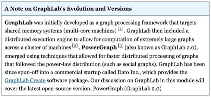
In this module, we present GraphLab, a variant graph-parallel distributed analytics engine that can efficiently and correctly execute both synchronous and asynchronous MLDM problems and others. GraphLab is also well suited to graphs that show power-law distribution. In this module,

1. We first discuss the data structure that should be used in storing input graphs for GraphLab to consume, process and show how input graphs flow through the GraphLab engine, starting from getting consumed to generating results.
2. We identify the architectural model of GraphLab.
3. We present the programming model employed by GraphLab and the consistency mechanisms supported for protecting shared data from read-write/write-write conflicts.
4. We discuss the asynchronous computation model that underlies GraphLab.
5. We examine GraphLab's fault-tolerance techniques.

References

1. J. Gonzalez, Y. Low, H. Gu, D. Bickson, and C. Guestrin (October, 2012). "PowerGraph: Distributed Graph-Parallel Computation on Natural Graphs." In Proc. of the 10th USENIX Conference on Operating Systems Design and Implementation.

Data Structure and Graph Flow

Data Structure and Graph Flow in Graphlab

Developed by Carnegie Mellon University, GraphLab provides an example of graph-parallel distributed analytics engines for the cloud. As with any graph-parallel engine, GraphLab assumes input problems modeled as graphs, in which vertices represent computations and edges encode data dependencies or communication.

In GraphLab, graphs are initially stored as files in an underlying distributed storage layer, such as HDFS, as shown in Figure 5.46. GraphLab is composed of two phases:initialization and execution. During initialization, the GraphLab engine reads input graph files from the underlying storage and divides them into multiple partitions that can be distributed among multiple machines in the cluster. During the execution phase, each machine runs the user-defined computation on the graph vertices, transmitting updates and iterating until some convergence condition is met.

Initialization Phase

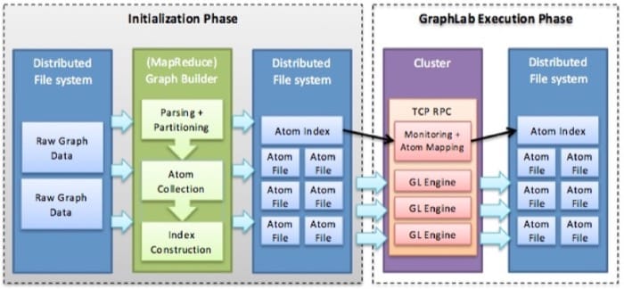
In the first phase, the input graph is divided into k partitions, called atoms, where k is much larger than the number of cluster machines. As demonstrated in Figure 5.46, atoms can be constructed either sequentially or using parallel loading techniques, including MapReduce. GraphLab does not store the actual vertices and edges in atoms but rather the commands to generate them, in the form of a journal. This allows GraphLab to reconstuct portions of the graph in case of node failures. In addition, GraphLab maintains in each atom information about its neighboring vertices and edges. This information, denoted in GraphLab as ghost vertices, provides a caching capability for efficient adjacency data accessibility as explained in the section The Programming Model.

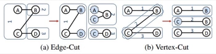
The graph can be partitioned across the cluster machines in a number of ways (Figure 5.47). A simple technique is edge-cut, where graph is partitioned along each vertex (Figure 5.47(a)). Each vertex is randomly assigned to a machine along with all its associated edges. As a result, ghost vertices are generated so that edges can be associated with a vertex that is not in a particular machine. However, for graphs with power-law distribution of edges, this means that the edge-cut partitioning will be unbalanced and some machines will be more loaded than others (due to the star-like motifs of a small number of vertices). To deal with such graphs, GraphLab uses a novel technique (known as Greedy Vertex Cuts) to partition high-degree vertices across machines in order to distribute the computation more effectively. Vertices of high degree are replicated across machines, with each machine receiving a subset of the edges for that vertex (Figure 5.47(b)). The machine that holds a given edge for a vertex is decided using the following algorithm:

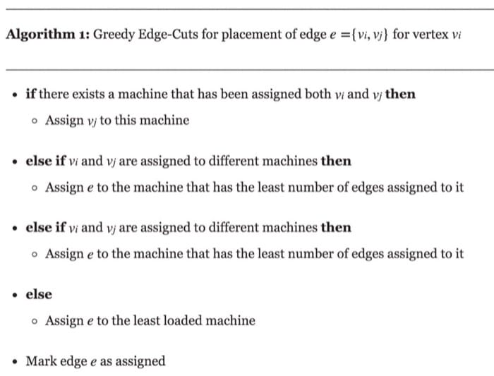
Loading of these partitions can be done in a distributed and coordinated manner, which ensures that the assignment of vertices and edges across the cluster is optimal, but the time taken to load is much higher than a random placement. On the other hand, random placement will lead to unbalanced load and loss of locality. A compromise between these two approaches, wherein each machine estimates the assignments of the edges and vertices in the cluster, is a tradeoff suggested in [3] .

Users, however, do need to store graphs in formats that can be consumed and parsed by GraphLab during its initialization phase. Clearly, this depends on the underlying storage layer and the parsing engine that GraphLab employs. For instance, if MapReduce is used to read and parse input graph files from HDFS, the input graph files have to be formatted using MapReduce's key-value data structure.

Generating atoms for a given input graph completes the first phase of GraphLab's partitioning strategy. Subsequently, the engine stores the connectivity structure and atom locations in an index file denoted also as a meta-graph (Figure 5.46). The atom index file encompasses k vertices, each corresponding to an atom, and edges encoding connectivity among them. In the second phase, the atom index file is split evenly across cluster machines. Atoms are then loaded by cluster machines, and each machine constructs its partition(s) of the given graph by executing the journal in each of its assigned atoms. By generating partitions from atom journals (and not directly mapping partitions to cluster machines), GraphLab allows future graph changes to be simply appended as journal commands, without needing to repartition the entire graphs. Furthermore, the same graph atoms can be reused for different cluster sizes by simply re-dividing the corresponding atom index file and re-executing atom journals, thus repeating only the second partitioning phase.

Construction of graph partitions at cluster machines concludes GraphLab's initialization phase, and the execution phase begins.

Execution Phase

As shown in Figure 5.46, each cluster machine runs an instance of the GraphLab engine, which incorporates two main parts: the data graph, and the user-defined functions that operate on the data graph. The data graph represents the user program state at a cluster machine and includes a directed graph G=(V,E,D), where V is the set of vertices, E is the set of edges, and D is the user-defined data (e.g., parameters, user input data, and even statistical data). In GraphLab, data is associated with both vertices and edges.

Computation is then represented as a stateless program that is executed on each vertex of the graph in parallel. This program consists of three distinct phases namely,Gather, Apply, and Scatter (GAS).

Gather Phase: In the gather phase, each vertex (henceforth refferred to as the central vertex) gathers information from adjacent vertices and edges. GraphLab can then apply a user-defined aggregation or sum operation:

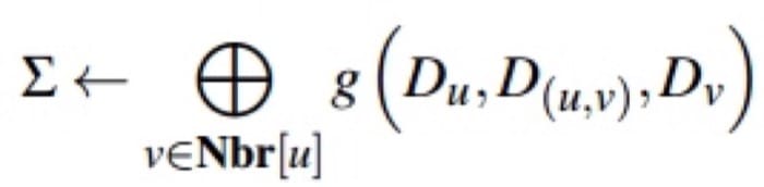
In the equation above Du, Dv, and D(u,v) denote values and metadata for vertices u,v and edge(u,v) respectively. The user defined sum (⊕) operation must be commutative and associative and can range from a numerical sum to the union of the data on all neighboring vertices and edges.

Apply Phase: In the apply phase, the resulting value ∑ is used to update the value of the central vertex:

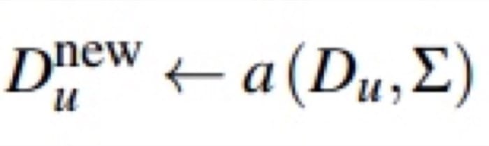
Scatter Phase: Finally in the scatter phase, the new value of the central vertex is sent to all adjacent vertices:

With the end of the scatter operation, one iteration of the computation for the vertex is complete.

The GAS functions are executed on a set of active vertices on every iteration. During the initial iteration, all vertices are placed in the set of active vertices, and based on the logic of the GAS functions, a vertex can mark one of its neighbors as active, so that it can be computed upon in the next iteration.

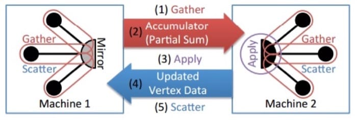
Figure 5.48 illustrates the resulting communication pattern of employing the GAS functions on a graph partitioned using the Greedy Edge-Cuts algorithm described earlier. Gather functions run locally on each machine that contains the ghost of a vertex. During the accumulation, these gathered values are sent to the machine that has the master copy of the vertex, where it can compute the function defined in the apply stage. Finally, the updated vertex data is copied to all machines that have ghost copies of the vertex and the scatter function is executed to propagate values to the adjacent vertices.

Delta Caching: There are situations where a vertex program will be triggered (made active) because of a change in only few of its neighbors. When the vertex is triggered, it will execute a gather operation from all neighbors, many of whom have not executed and hence will return values which are unchanged since the last time this particular vertex ran. GraphLab introduces a subtle optimization called delta caching, where the result of gather operations from all of the neighbors of a vertex are cached at that vertex. During the scatter operation that is run at the neighbouring vertices, an optional parameter, Δa can be sent, summarizing the change in the value of variable a between iterations. This value can be used to bypass the gather phase and added to the cached value of a to speed up execution.

References

1. Y. Low, J. Gonzalez, A. Kyrola, D. Bickson, C. Guestrin, and J. M. Hellerstein (2010). "GraphLab: A New Parallel Framework for Machine Learning." Conference on Uncertainty in Artificial Intelligence (UAI).
2. Y. Low, J. Gonzalez, A. Kyrola, D. Bickson, C. Guestrin, and J. M. Hellerstein (2012). "Distributed GraphLab: A Framework for Machine Learning and Data Mining in the Cloud." PVLDB.
3. J. Gonzalez, Y. Low, H. Gu, D. Bickson, and C. Guestrin (October, 2012). "PowerGraph: Distributed Graph-Parallel Computation on Natural Graphs." In Proc. of the 10th USENIX Conference on Operating Systems Design and Implementation.

The Architectural Model

The Architectural Model of GraphLab

When GraphLab is launched on a cluster, one instance of its engine is started on each machine, as shown previously in Figure 5.46. All engine instances are symmetric; that is, they have the same capability. Moreover, they all communicate directly with each other using a customized, asynchronous Remote Procedure Call (RPC) protocol over TCP/IP. The first triggered engine instance, however, will have the additional responsibility of serving as monitor/master engine, although instances on other machines will still work and communicate directly without coordination from the master. This arrangement makes GraphLab a peer-to-peer system.1 The master engine computes the atom mapping based on the atom index file and instructs corresponding engine instances to load their assigned atoms. Subsequently, all instances load their atoms in parallel. Each engine then executes the journal in each of its assigned atoms, generating a partition of the input graph (see the section The Data Structure and Graph Flow in this module) and runs the user-defined program specified in Algorithm 1. As each engine loads its atoms, generates its partitions, executes code, and schedules vertices without polling the master engine, GraphLab employs a push-based, thread-scheduling strategy (see the section Models for Distributed Programming). As a consequence of employing a symmetric design, GraphLab exposes high scalability and precludes centralized bottlenecks and single points of failure (SPOFs), unlike both Hadoop MapReduce 1.0 and Pregel.

Recall that in peer-to-peer systems, a master may be adopted, but only for purposes like monitoring the system and/or injecting commands. Processes in such systems work and communicate directly without having to contact master machines.

The Programming Model

The GraphLab Programming Model

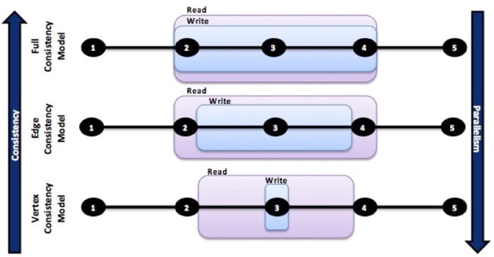
Recall from the data model of GraphLab, graphs are partitioned between multiple machines. During the execution of the GAS functions on each vertex, there exists potential for read-write and write-write conflicts among vertices that share scope. The GraphLab engine synchronizes shared data accesses and ensures consistent parallel execution. In particular, GraphLab supports different graph execution engines, each with different levels of consistency, allowing users to choose an engine appropriate for correctness and performance in their applications. The different notions of consistency offered by GraphLab through its various engines are: full consistency, edge consistency, and vertex consistency. As shown in Figure 5.49, under full consistency, the update function at each vertex (vertex 3) has an exclusive read-write access to its own vertex, adjacent edges, and adjacent vertices (its entire scope). While this arrangement guarantees strong consistency and full correctness, it limits parallelism and, consequently, performance. Vertices in many MLDM algorithms, however, really do not require exclusive read-write access to their entire scope. For instance, the PageRank algorithm requires only read access to neighboring edges and vertices.

Thus, to increase parallelism and support a broader range of consistency settings that suit various MLDM applications, GraphLab includes notions of edge consistency and vertex consistency. Under edge consistency, the update function at a vertex has an exclusive read-write access to its vertex and adjacent edges, yet a read-only access to adjacent vertices. Clearly, this protocol relaxes consistency and enables a superior leverage of parallelism. Under vertex consistency, the update function at a vertex has exclusive write access only to its own vertex, thus allowing all update functions to run simultaneously. This capability provides the maximum possible parallelism but, in return, the most relaxed consistency. GraphLab users can choose an engine that balances performance with the required consistency model they find convenient for their applications.

As part of its shared-memory view, GraphLab stores ghosts, the adjacency information/data of each vertex (see the section The Data Structure and Graph Flow), in local memories. A vertex ghost ensures that the vertex's update function has direct memory access to all data within its scope.

References

1. Yucheng Low and Joseph Gonzalez and Aapo Kyrola and Danny Bickson and Carlos Guestrin and Joseph M. Hellerstein (2010). "GraphLab: A New Parallel Framework for Machine Learning." Conference on Uncertainty in Artificial Intelligence (UAI).
2. Low, Y., Gonzalez, J., Kyrola, A., Bickson, D., Guestrin, C., and Hellerstein, J. M. (2012). "Distributed GraphLab: A Framework for Machine Learning and Data Mining in the Cloud." PVLDB.
3. J. Gonzalez, Y. Low, H. Gu, D. Bickson, and C. Guestrin (October, 2012). "PowerGraph: Distributed Graph-Parallel Computation on Natural Graphs." In Proc. of the 10th USENIX Conference on Operating Systems Design and Implementation.

The Computation Model

As discussed on the previous page, GraphLab supports multiple engines which can execute the vertex functions either synchronously or asynchronously. The three engines currently supported by GraphLab are the following:

• Synchronous Engine
• Asynchronous Engine
• Asynchronous Engine - Serializable

Synchronous Engine

The synchronous engine executes the gather, apply and scatter (GAS) phases in order for each of the active vertices assigned to a machine. Once a machine completes updating all the vertices assigned to it for a particular iteration, it waits for the next iteration. Vertices that are activated in each iteration are scheduled for execution for the next iteration. In this execution mode, GraphLab actually executes the computation in Bulk-Synchronous (BSP) fashion, similar to systems such as Pregel. As a result, the computation performed by the synchronous engine is guaranteed to follow the full consistency model as discussed in the previous page.

The Synchronous engine can perform extremely poorly when executing MLDM algorithms because a phase/stage/super-step during that execution cannot finish before the last task/vertex in that computation commits, and execution time of each phase/stage/super-step is determined by its slowest task/vertex (see the sectionIntroduction to Distributed Programming for the Cloud ).

Asynchronous Engine

Using the asynchronous engine, GraphLab executes active vertices as machines become available. Changes made to the vertex and edge data during the apply and scatter functions are immediately committed to the graph and made available for subsequent computation on neighboring vertices. The main benefit in using an asynchronous engine is in the elimination of waiting before the next iteration can proceed, which allows for increased parallelism and performance. The asynchronous engine executes vertex computations using the vertex consistency model as discussed in the previous page.

Although asynchronous engines can result in empirical and algorithmic gains for a range of common MLDM applications, they pose a critical challenge. In particular, asynchronous execution presents design and debugging complexities and can yield nondeterministic results [2] . For example, when statistical simulation is run asynchronously, there is a high potential for nondeterministic outcomes. If this condition is not carefully controlled, instability or even divergence can occur [8] . In certain applications, the increased parallelism of asynchronous execution is offset by the increased number of iterations required to achieve convergence.

Asynchronous-Serializable Engine

Graphlab provides a balanced tradeoff between the synchronous and asynchronous engines with the option of using the asynchronous-serializable engine. In this engine. GraphLab prevents adjacent vertices’ GAS functions from running concurrently by using fine-grained, parallel locking protocol, known as the Chandy-Misra [9] scheme. Using this scheme, a machine executing a vertex acquires locks on adjacent edges that are present on the machine (this is determined during the Greedy-Edge cut partitioning described earlier). The resulting execution is guaranteed to beserializable; i.e. there exists some serial ordering of execution whose results are equivalent to the results when executed using the asynchronous-seralizable engine. The asynchronous-serializable execution of a graph is equivalent to the edge consistency model as discussed in the previous page.

References

1. Y. Low, J. Gonzalez, A. Kyrola, D. Bickson, C. Guestrin, and J. M. Hellerstein (2012). "Distributed GraphLab: A Framework for Machine Learning and Data Mining in the Cloud." PVLDB.
2. J. Gonzalez, Y. Low, H. Gu, D. Bickson, and C. Guestrin (October, 2012). "PowerGraph: Distributed Graph-Parallel Computation on Natural Graphs." In Proc. of the 10th USENIX Conference on Operating Systems Design and Implementation.
3. D. P. Bertsekas and J. N. Tsitsiklis (1989). "Parallel and Distributed Computation: Numerical Methods." Prentice Hall.
4. J. Gonzalez, Y. Low, and C. Guestrin (2009). "Residual Splash for Optimally Parallelizing Belief Propagation." In AISTATS, vol. 5, pp. 177–184.
5. R. Neal and G. Hinton (1998). "A View of the EM Algorithm that Justifies Incremental, Sparse, and Other Variants." In Learning in Graphical Models, pp. 355–368.
6. A. G. Siapas (1996). "Criticality and Parallelism in Combinatorial Optimization." PhD thesis, Massachusetts Institute of Technology.
7. A. J. Smola and S. Narayanamurthy (2010). "An Architecture for Parallel Topic Models." PVLDB, 3(1):703-710.
8. J. Gonzalez, Y. Low, A. Gretton, and C. Guestrin (2011). "Parallel Gibbs Sampling: From Colored Felds to Thin Junction Trees." In AISTATS, vol. 15, pp. 324-332.
9. Chandy, K. M. and Misra, J. (1984). "The Drinking Philosophers Problem." ACM Trans. Program. Lang. Syst. 632--646 Pages.

Fault Tolerance

Fault Tolerance in GraphLab

To tolerate faults in the event of failures, GraphLab suggests using distributed checkpointing (see the section Main Challenges in Building Cloud Programs) and promotes two distributed checkpointing mechanisms: synchronous and asynchronous. To capture a distributed checkpoint, the synchronous mechanism suspends the entire execution of the update functions across cluster machines. By doing so, the mechanism flushes out all in-transit communication messages (induced internally by the engines) and takes a local checkpoint (snapshot) of all altered data at each machine since the last captured checkpoint. The captured local checkpoints collectively form a distributed checkpoint, which is then stored in files6 in the engine's underlying storage layer (e.g., HDFS). In case of a machine/engine failure, the distributed checkpoint can be exploited to restart execution.

Although synchronous checkpointing is simple, it introduces a major inefficiency by suspending the entire GraphLab execution to capture a distributed checkpoint. To address this weakness, the asynchronous mechanism specifies at each cluster machine a checkpointing update function that executes on each vertex, collecting snapshots covering the period since the last saved snapshot. At each machine, checkpointing update functions proceed as shown in algorithm 2. They are prioritized over regular update functions (used by GraphLab user programs) and follow the edge consistency model. Hence, when the scope of a vertex v is locked, as required by the edge consistency model, it remains so until algorithm 2 completes at v before proceeding to another vertex. This asynchronous mechanism is based on the Chandy-Lamport checkpointing strategy [1] and guarantees consistent distributed checkpoints. Finally, both synchronous and asynchronous checkpointing mechanisms are triggered by GraphLab at fixed intervals, computed as in Young's "A First Order Approximation to the Optimum Checkpoint Interval." [2]

With fault tolerance, we close our discussion on GraphLab. This engine employs graph-parallel, shared-memory, asynchronous, and peer-to-peer models. It supports three levels of consistency that trade off parallelism against consistency, allowing users to select—from full consistency, edge consistency, and vertex consistency—a level that suits their application needs. It further ensures serializability (requisite for many machine-learning and data-mining [MLDM] algorithms) with respect to the appropriate consistency model. GraphLab also suggests two types of asynchronous engines, Chromatic and Locking. The Chromatic engine executes vertices partially asynchronously, while the Locking engine executes vertices fully asynchronously. The Chromatic engine uses graph coloring and promotes the color-step concept, which is analogous to the super-step concept in the bulk synchronous parallel model. In essence, GraphLab with the Chromatic engine and the edge consistency model can mimic Pregel. Finally, to achieve fault tolerance, GraphLab suggests using synchronous and asynchronous distributed checkpointing.

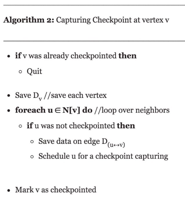
The distributed checkpoint consists of every local checkpoint captured at every cluster machine. Each local checkpoint can be stored in a file, and all files corresponding to local checkpoints can be associated together (in metadata) in order to indicate that they all belong to the same distributed checkpoint.

References

1. K. M. Chandy and L. Lamport (1985). "Distributed Snapshots: Determining Global States of Distributed Systems." ACM Trans. Comput. Syst., 3(1):63–75.
2. J. W. Young (1974). "A First Order Approximation to the Optimum Checkpoint Interval." Commun. ACM, 17:530–531.

An Example Application in GraphLab

In this section, we explore the abstraction of GraphLab by walking through the PageRank example. The PageRank algorithm is a well-known technique proposed by Google. It is used by Google to rank the importance of website pages returned by their search engine. Using the assumption that more important websites are likely to receive more links from other important websites, it determines the importance of a page by counting the number and quality of links pointed to that page.

PageRank has various implementations, but its idea can be demonstrated with the following equation:

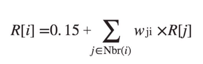
where R[i] represents the PageRank value of page i, Nbr(i) is the set of pages pointing to page i and wji is a weight associated with this link, which is normally defined as the inverse of page j’s outdegree.

As you may have noticed, the above equation is recursive, the PageRank value of different pages may mutually dependent on each other. Therefore, the computing process of PageRank often starts with a set of initial values, and each page iteratively applies the above equation to update its value until reaching convergence.

To perform this algorithm with GraphLab, we first map the problem to a graph-based abstraction. For PageRank, this should be intuitive; the vertices of the graph correspond to pages and edges correspond to links of the pages. We also add a per-vertex parameter, the rank of the page, denoted as R[i]. Now that the data is represented in GraphLab, we decompose the operation expressed in the PageRank equation to Gather, Apply, Scatter steps in GraphLab’s abstraction:

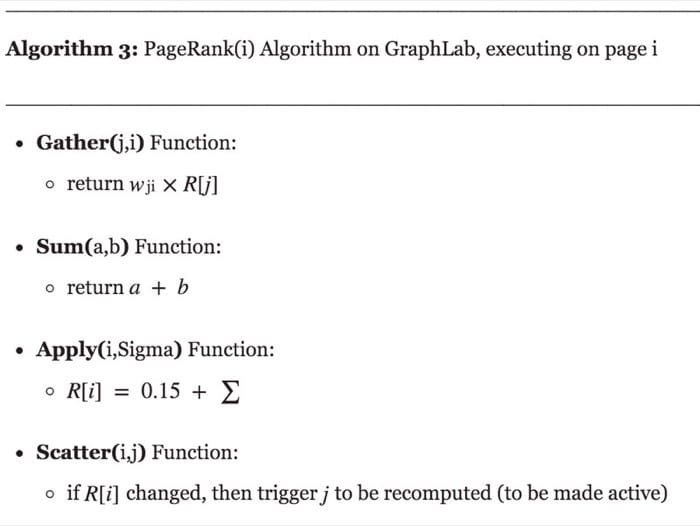
In the Gather phase, page i goes through each of its in-edges, and gathers the corresponding values from its neighbors. The gathered values will be accumulated using the Sum function, which simply adds all the in-edge values in this algorithm. Next, page i performs Apply function to update its PageRank value to the sum of 0.15 and the aggregated result. Finally, it checks if the updated PageRank is different from the previous one, and goes through each out-edge to trigger the recomputation of its neighbors if the PageRank value is changed. Pagerank will iteratively run the GAS functions defined above for all active vertices until the values do not change beyond a certain threshold. When there are no more active vertices, the algorithm is said to haveconverged to the required result.

Summary

Comparison of the Various Distributed Analytics Engines

Here we conclude our discussion of distributed analytics engines for the cloud in which we presented Hadoop MapReduce, Spark, and GraphLab as effective and popular frameworks for distributed programming. Each of these three engines take care of the following aspects of distributed computation on behalf of the user:

• Design and implement an appropriate programming model (message passing or shared memory) and resolve all the associated synchronization and consistency issues
• Develop the computation model (synchronous or asynchronous)
• Specify the parallelism model (graph parallel, data parallel, iterative) and encode the necessary partitioning and mapping algorithms
• Design the underlying architectural structure (master-slave or peer to peer)
• Implement an effective task/vertex scheduling strategy (push based or pull based)

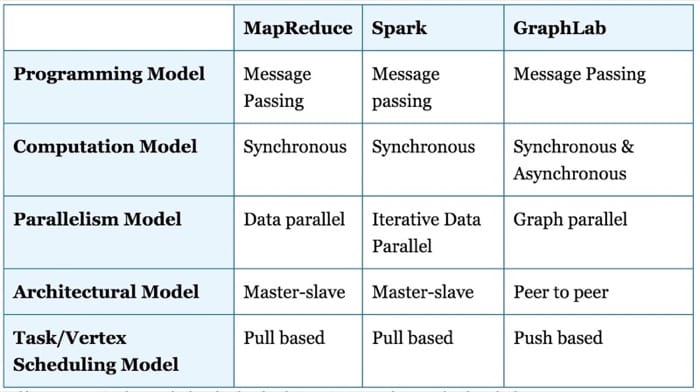
Table 5.4 compares the three engines on each of these dimensions: MapReduce and Spark employ a data-parallel design, while GraphLab programs are executed in graph-parallel fashion. MapReduce and Spark both suggest synchronous computation models, while GraphLab make both synchronous and asynchronous engines available to the user. MapReduce suits applications relatively loosely connected or embarrassingly parallel (with little or no dependency/communication between parallel tasks) and that involve noniterative computations with large data volumes. Spark optimizes the MapReduce model for applications that need to iteratively apply Map and Reduce functions to data. On the other hand, GraphLab fits more strongly connected applications (with high degrees of dependency between parallel tasks/vertices) and that involve iterative computations with little data per a task/vertex. GraphLab also includes specific optimizations that allow for balanced and efficient distribution of work among nodes processing graphs that have power-law distribution, such as social and web-graphs.

Summary

Distributed Analytics Engines for the Cloud: GraphLab Summary

• GraphLab is a graph-parallel distributed analytics engine designed for machine-learning and data-mining (MLDM) applications.
• GraphLab programs are executed in two phases: the initialization phase and the execution phase.
• Computation in GraphLab is performed via a user-defined Gather, Apply, Scatter (GAS) operations which updates the values related to a vertex.
• GraphLab differs from Pregel in that the computation model is support both synchronous and asynchronous computation.
• GraphLab nodes are organized in a peer-to-peer fashion, although the first launched node is designated as the master engine and is used to monitor the system.
• GraphLab supports tunable consistency under the full, edge, and vertex consistency models through the use of different engines, in the order of decreasing consistency and increased parallelism.
• GraphLab provides three engines: synchronous, asynchronous and asynchronous-serializable.
• To achieve fault tolerance, GraphLab suggests using synchronous and asynchronous distributed checkpointing.
• MapReduce and Spark are regarded as a data-parallel engines, while GraphLab is characterized as a graph-parallel engine.
• MapReduce suits more loosely connected/embarrassingly parallel applications, Spark suits iterative computations, and GraphLab suits more strongly connected applications that can be expressed in the graph abstraction.