云计算 阅读材料 19 Distributed Analytics Engines for the Cloud - MapReduce

MapReduce is a data-parallel framework, originally created by Google, for processing big-data applications on large suites of computers. The system attempts to decrease interprocess communication by moving computation towards data. It also transparently tolerates data and computation faults, both highly probable in large-scale cloud settings.

---

Developers, consequently, recognize MapReduce for its scalability, fault tolerance, and elasticity. Google utilizes it to process 20PB of data per day, and Amazon recently enhanced its Web Services with Amazon Elastic MapReduce (EMR), effectively a pay-as-you-go cloud analytics engine that enables businesses, researchers, data analysts, and developers to process vast amounts of data easily and cost effectively.

Since its debut, MapReduce has been frequently associated with Hadoop, an open-source implementation of MapReduce. Academic, government, and industrial use of Hadoop is growing rapidly. For instance, Yahoo! uses it for around 80% to 90% of its jobs, and others, such as Facebook and Microsoft, have also advocated the framework. Amazon EMR rests on a Hadoop MapReduce engine hosted in Amazon Elastic Compute Cloud (Amazon EC2) and Amazon Simple Storage Service (Amazon S3). Academia currently uses Hadoop for seismic simulation, natural-language processing, and Web data mining, among other applications. [10]

Hadoop MapReduce performs most of the labor involved in implementing cloud programs through three main strategies:

• It automatically breaks down jobs into distributed tasks to effectively exploit task parallelism.
• It considers data locality and variations in overall system workloads to schedule jobs and tasks efficiently at participating cluster nodes.
• It transparently tolerates both data and task failures.

References

1. Big-Data Analytics Predictions for 2011. http://tdwi.org/articles/2011/03/16/big-data-analytics-predictions.aspx/.
2. J. Dean and S. Ghemawat (Dec. 2004). "Mapreduce: Simplified Data Processing on Large Clusters." OSDI.
3. Amazon Elastic MapReduce. http://aws.amazon.com/elasticmapreduce/.
4. H. Herodotou, H. Lim, G. Luo, N. Borisov, L. Dong, F. B. Cetin, and S. Babu (2011). "Starfish: A Self-Tuning System for Big Data Analytics." CIDR.
5. Z. Fadika and M. Govindaraju (Dec. 2010). "LEMO-MR: Low Overhead and Elastic MapReduce Implementation Optimized for Memory and CPU-Intensive Applications." IEEE 2nd Int. Conf. on Cloud Computing Technology and Science (CloudCom).
6. Hadoop. http://hadoop.apache.org/.
7. N. B. Rizvandi, A. Y. Zomaya, A. J. Boloori, and J. Taheri (2011). "Preliminary Results: Modeling Relation between Total Execution Time of MapReduce Applications and Number of Mappers/Reducers." Tech. R. 679, The University of Sydney.
8. S. Ibrahim, H. Jin, L. Lu, S. Wu, B. He, and L. Qi (Dec. 2010). "LEEN: Locality/Fairness-Aware Key Partitioning for MapReduce in the Cloud." CloudComm.
9. M. Hammoud and M. F. Sakr (2011). "Locality-Aware Reduce Task Scheduling for MapReduce." CloudCom.
10. M. Zaharia, A. Konwinski, A. Joseph, R. Katz, and I. Stoica (2008). "Improving Mapreduce Performance in Heterogeneous Environments." OSDI.

Hadoop MapReduce Programming Model

Hadoop presents MapReduce as an analytics engine and, "under the hood," employs the Hadoop Distributed File System (HDFS). HDFS mimics the Google File System (GFS) and partitions input datasets into fixed-size chunks (blocks), distributing them on participating cluster nodes. By default 64MB, each HDFS block can be configured differently by users. Jobs can subsequently process HDFS blocks in parallel at distributed machines, thus exploiting the parallelism enabled by partitioning datasets. MapReduce breaks jobs into multiple tasks denoted as map and reduce tasks. All map tasks are encapsulated in what is known as the map phase, and reduce tasks are encompassed in what is called the reduce phase. The map phase can have one or many map tasks, and the reduce phase can have zero or many reduce tasks. When a MapReduce job includes no reduce tasks, it is referred to as "reduce-less."

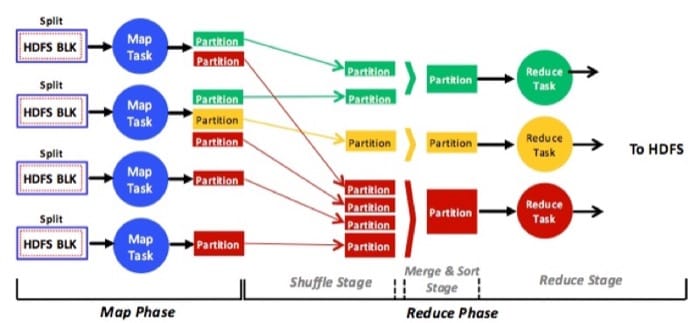
Figure 5.15 demonstrates a full, although simplified, view of the MapReduce analytics engine. Map tasks operate on distributed HDFS blocks, and reduce tasks operate on map tasks' output, denoted as intermediate output, or partitions. Each map task processes one or many distinct HDFS blocks (more on this shortly), and each reduce task processes one or many partitions. In a typical MapReduce program, the map task that is run across all the input HDFS blocks is the same and the reduce task run across all the partitions is also the same. Therefore, within a specific Map or Reduce phase, MapReduce jobs can considered to be in the single program, multiple data (SPMD) category (see the section Data Parallel and Graph Parallel Computations).

Map and reduce tasks consume different data, operating independently and in parallel only in their respective phases. That is, tasks in the same phase never communicate (send or receive messages), and the only communication in MapReduce occurs explicitly (through the help of the MapReduce framework) between different tasks in different phases. Specifically, map tasks generate new partitions in the map phase, and the Hadoop engine itself transfers partitions (over the network) to the reduce tasks in the reduce phase in a process called shuffling. The rationale behind such a strategy is that Hadoop would not scale to large clusters (hundreds or thousands of nodes) if tasks were allowed to communicate arbitrarily. Instead, all communication occurs only between the map and the reduce phases and under the full control of the engine itself (not the tasks). Therefore a typical program running in the MapReduce variant can be considered to be a special case of the of the Message Passing model, as tasks do not have access to a common shared memory, but rely on messages being passed by the framework between the Map and Reduce synchronisation barrier.

References

1. Hadoop
2. S. Ghemawat, H. Gobioff, and S. T. Leung (Oct. 2003). "The Google File System." SOSP.
3. S. Chen and S. W. Schlosser (May 2008). "Map-Reduce Meets Wider Varieties of Applications." Intel Research Pittsburgh, Tech. Rep. IRP-TR-08-05.

The Data Structure and Flow

When a user submits a job, the associated HDFS data blocks are loaded and fed to the map tasks in the map phase (see Figure 5.15). Each map task processes one or many HDFS blocks encapsulated in what is called a split. A split can contain one or many references (not actual data) to one or many HDFS blocks. Split size, how many HDFS blocks a split references, is a configurable parameter. Each map task is always responsible for processing only one split. Thus, the number of splits dictates the number of map tasks in a MapReduce job, which in return, dictates the overall map parallelism. If a split points to only one HDFS block, the number of map tasks becomes equal to the number of HDFS blocks. For data-locality reasons, a common practice in Hadoop is to have each split encapsulate only one HDFS block. Specifically, MapReduce attempts to schedule map tasks in proximity to input splits so as to diminish network traffic and improve application performance (see the section Fault Tolerance). Hence, when a split references more than one block, the probability of these blocks existing at the same node where the respective map task will run becomes low. This leads to a network transfer of at least one block (64MB by default) per map task. With a one-to-one mapping between splits and blocks, however, a map task can run at a node at which the required block exists and, subsequently, leverage data locality and reduce network traffic.

In the presence of a reduce phase, map tasks store partitions on local disks (not in HDFS) and hash them to designated reduce tasks. Each reduce task collects (shuffles) its corresponding partitions from local disks, merges and sorts them, runs a user-defined reduce function, and stores the final result in HDFS. Thus, the reduce phase is usually broken into shuffle, merge and sort, and reduce stages, as shown in Figure 5.15. In the absence of a reduce phase, map tasks write their outputs directly to HDFS. Figure 5.15 shows that reduce tasks can receive varied numbers of partitions with different sizes. This phenomenon is called partitioning skew and has some effects on reduce task scheduling, as discussed in the section Fault-Tolerance.

Figure 5.15 demonstrates a simplified view of what the Hadoop MapReduce engine actually does. For instance, MapReduce overlaps the map and the reduce phases for performance reasons. In particular, reduce tasks are scheduled after only a certain percentage (by default 5%) of map tasks complete so as they can gradually start shuffling their partitions. Specifically, the shuffle and the merge and sort stages execute simultaneously so that partitions are continuously merged while being fetched. The rationale behind such a strategy is to interleave execution of map and reduce tasks and enhance, accordingly, the turnaround times of MapReduce jobs. Such an interleaving technique is commonly called the early shuffle technique.

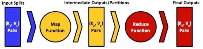
MapReduce has been inspired by functional languages so that programmers write functional-style code comprising sequential map and reduce functions that are submitted as jobs to the MapReduce engine. The engine transforms jobs into map and reduce tasks, distributing and scheduling them at participating cluster nodes. Map and reduce function inputs and outputs are always structured as key-value pairs, and dataflow follows the general pattern shown in Figure 5.16. Typically, the map input key and value types, K1-V1, will differ from the function's output key-value types, K2 andV2. The reduce input key and value types, K2 and V2, however, should match map function outputs. The reduce function allows aggregating values together, so it usually receives an iterator (list) of input values from multiple map tasks. It then applies the user-defined reduce function on these values collectively, possibly returning a new key-value(s) types, K3 and V3. A key from a map task can appear at only one reduce task, while a reduce task can receive and process keys from one or many map tasks. This property is guaranteed by the MapReduce engine (specifically the hashing function used in partitioning the map output). Last, an extra function, called the combiner function, can be introduced at the map function output where it acts just like a reduce function. In this case, the combiner function's output will subsequently form the input to the reduce function.

The number of HDFS blocks of a job can be computed by dividing the job's dataset size by the configurable HDFS block size.

Each reduce task processes one or many values produced by one or many map tasks.

References

1. S. Ibrahim, H. Jin, L. Lu, S. Wu, B. He, and L. Qi (Dec. 2010). "LEEN: Locality/Fairness-Aware Key Partitioning for MapReduce in the Cloud." CloudComm.
2. M. Hammoud and M. F. Sakr (2011). "Locality-Aware Reduce Task Scheduling for MapReduce." CloudCom.
3. M. Zaharia, A. Konwinski, A. Joseph, R. Katz, and I. Stoica (2008). "Improving Mapreduce Performance in Heterogeneous Environments." OSDI.
4. Hadoop. http://hadoop.apache.org/docs/r1.0.4/hdfs_design.html.
5. S. Ghemawat, H. Gobioff, and S. T. Leung (Oct. 2003). "The Google File System." SOSP.
6. S. Chen and S. W. Schlosser (May 2008). "Map-Reduce Meets Wider Varieties of Applications." Intel Research Pittsburgh, Tech. Rep. IRP-TR-08-05.
7. M. Hammoud, M. S. Rehman, and M. F. Sakr (2012). "Center-of-Gravity Reduce Task Scheduling to Lower MapReduce Network Traffic." CLOUD.
8. J. Gray, S. Chaudhuri, A. Bosworth, A. Layman, D. Reichart, M. Venkatrao, and H. Pirahesh (1997). "Data Cube: A Relational Aggregation Operator Generalizing Group-by, Cross-tab, and Sub-totals." Data Mining and Knowledge Discovery.

Examples WordCount, Sort, and Sobel

MapReduce Program Examples

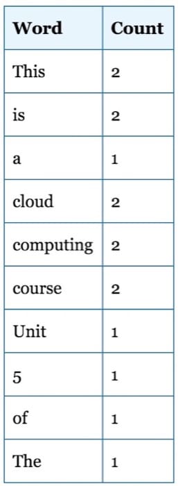
As a simple MapReduce example, we can write a job/program that counts the times that each word appears in a file or a set of files. For instance, if we assume two files, Aand B, with contents "This is a cloud computing course" and "This is Unit 5 in the cloud computing course," we would expect an output similar to what is shown in Table 5.1. Such a program is commonly called WordCount. The WordCount program is included in the Hadoop distribution and is readily available for running and testing. It represents a large spectrum of text-processing algorithms in big-data applications. As such, many consider it a state-of-the-art benchmark workload for evaluating Hadoop's efficiency. The original MapReduce paper has indeed used WordCount as a benchmark workload. Yahoo! uses it also for evaluating Hadoop on its data centers.

MapReduce programs can be written in the Java programming language. To write a WordCount program (or MapReduce programs in general), we usually start by defining input and output formats for the map and reduce functions. Since we are dealing with key-value pairs, we need only specify the actual keys and values that input and output files will contain and their types (e.g., string or numerical). A job's input (the input dataset), being one or a million files, must always exhibit the same format. Similarly, a job's output files must always expose the same format, which might differ from the input formats.

Input and output formats can be arbitrary, line-based logs, for example, or images, videos, multiline records, or something totally different. Hadoop can process any file format, from flat text, through binary, to structured databases. To arrange this, users can override Hadoop's InputFormat (default TextInputFormat) and OutputFormat(default TextOutputFormat) classes. The former defines how input files are read as key-value pairs and constructs the corresponding input splits for map tasks. The Hadoop engine spawns one map task per each input split thus generated. TheOutputFormat class similarly defines how key-value pairs are written by reduce tasks as output files to HDFS (watch Video 5.1 for a detailed illustration on how theInputFormat and the OutputFormat classes are used in Hadoop MapReduce).

The default I/O subclasses are suitable for text processing. Specifically,TextInputFormat enables reading text files, with the byte offset of a line being a key and the actual line content being a value. TextOutputFormat allows writing files as key-value3 text pairs. Other formatting classes, such as theSequenceFileInputFormat and the SequenceFileOutputFormat classes, are shipped with Hadoop and allow reading and writing binary files. In addition, Hadoop users can always implement custom input and output format classes tailored for their input datasets. More information on how to do that can be found on the Yahoo! Hadoop Tutorial and in White's "Hadoop: The Definitive Guide."

Video 5.1: MapReduce Internals

Our WordCount example assumes text file inputs. Thus, we can directly use theTextInputFormat class, with a key being the byte offset of a line in a file and a value being the line content itself. Furthermore, we can directly use the TextOutputFormatclass, with a key being a word encountered in the input dataset and a value being the frequency of the word. The key type can be set to Java Long (LongWritable in Hadoop) and the value type to Java String (Text in Hadoop). The reduce function should receive words from the map tasks as keys and the digit 1 per each word as values,4 so the key type will be that of words (Text) and the value type that of the unit digit (Java Integer, IntWritable in Hadoop). All that remains is the logic of the map and the reduce functions. For the map function, input splits should be parsed and each word emitted with a count of 1. In the reduce function, each word received can be simply output as is along with its frequency, computed after aggregating all the 1s received with that word.5 Figure 5.17 shows our complete WordCount example code for the new Java MapReduce API released in Hadoop 0.20.0.

import java.io.IOException;
import java.util.*;
import org.apache.hadoop.fs.Path;
import org.apache.hadoop.conf.*;
import org.apache.hadoop.io.*;
import org.apache.hadoop.mapreduce.*;
import org.apache.hadoop.mapreduce.lib.input.FileInputFormat;
import org.apache.hadoop.mapreduce.lib.input.TextInputFormat;
import org.apache.hadoop.mapreduce.lib.output.FileOutputFormat;
import org.apache.hadoop.mapreduce.lib.output.TextOutputFormat;

public class WordCount {

    public static class WCMap extends Mapper<LongWritable, Text, Text,
    IntWritable> {
        private final static IntWritable one = new
                IntWritable(1);
        private Text word = new Text();

        public void map(LongWritable key, Text value, Context context) throws
        IOException, InterruptedException {
            String line = value.toString();
            StringTokenizer tokenizer = new StringTokenizer(line);

            while (tokenizer.hasMoreTokens()) {
                word.set(tokenizer.nextToken());
                context.write(word, one);
            }
        }
    }

    public static class WCReduce extends Reducer<Text, IntWritable, Text,
    IntWritable> {

        public void reduce(Text key, Iterable<IntWritable> values, Context
        context)
                throws IOException, InterruptedException {
            int sum = 0;
            for (IntWritable val : values) {
                sum += val.get();
            }
            context.write(key, new IntWritable(sum));
        }
    }

    public static void main(String[] args) throws Exception {
        Configuration conf = new Configuration();

        Job job = new Job(conf, "wordcount");

        job.setOutputKeyClass(Text.class);
        job.setOutputValueClass(IntWritable.class);

        job.setMapperClass(WCMap.class);
        job.setReducerClass(WCReduce.class);

        job.setInputFormatClass(TextInputFormat.class);
        job.setOutputFormatClass(TextOutputFormat.class);

        FileInputFormat.addInputPath(job, new Path(args));
        FileOutputFormat.setOutputPath(job, new Path(args));

        job.waitForCompletion(true);
    }
}

Figure 5.17: The WordCount code using the new Java MapReduce API released in Hadoop 0.20.0

As Figure 5.17 shows, programmers need create only two sequential functions, map and reduce, encapsulated in two (inner) classes: in this case, the WCMap and theWCReduce inner classes. The WCMap inner class extends the Mapper class and overrides its map() function. The Mapper class maps given input key-value pair types (LongWritable and Text) to a set of output key-value pair types (Text andIntWritable). Output key-value pair types defined in the Mapper class should always match the input key-value pair types in the Reducer class. The WCReduce inner class extends the Reducer class and overrides its reduce() function. In addition to defining the input key-value pair types, the Reducer class defines the output key-value pair types (Text and IntWritable) that will be used by reduce tasks to generate the final results.

The map() and the reduce() functions in the WCMap and the WCReduce inner classes incorporate the actual logic of the WordCount program. The Context parameter in both functions performs I/O writes to local disks and HDFS. The main() function sets up a job to execute the WordCount program on a set of input files using theaddInputPath() function. It also specifies where the output files are placed on HDFS using the setOutputPath() function. In the main() function, setOutputKeyClass()and setOutputValueClass() specify the key-value pair types emitted by reduce tasks and assume, by default, that these types match the map task output key-value types. If this is not the case, the main() function should also call setMapOutputKeyClass()and setMapOutputValueClass() to specify map task output key-value types. To set the input and output formats, the functions setInputFormatClass() andsetOutputFormatClass() are called. Finally, the setMapperClass() and thesetReducerClass() functions are used to set the job's constituent inner map and reduce classes, WCMap and WCReduce. Video 5.2 discusses Sort, another classical MapReduce example, and Video 5.3 presents Sobel, an image-processing, edge-detection example.

Video 5.2: Sort in MapReduce Alternate Version

Video 5.3: Image Processing in MapReduce Alternate Version

Note that this is a tab space (not a single space) between the key and the value.

The digit 1 per a word, W, is output to indicate that W has appeared in an input split. This allows the reduce task, which receives W, to simply increment its counter for W.

Each reduce task can receive multiple words from multiple map tasks, but each word appears at only one reduce task.

References

1. J. Dean and S. Ghemawat (Dec. 2004). "MapReduce: Simplified Data Processing on Large Clusters." OSDI.
2. M. Zaharia, A. Konwinski, A. Joseph, R. Katz, and I. Stoica (2008). "Improving MapReduce Performance in Heterogeneous Environments." OSDI.
3. Hadoop
4. T. White (2011). "Hadoop: The Definitive Guide 2nd Edition." O'Reilly.

The Computation and Architectural Models

The Computation Model

MapReduce jobs, like all distributed programs, can embody either a synchronous or asynchronous computation model (see the section Synchronous and Asynchronous Distributed Programs). During each phase and stage, MapReduce tasks execute numerous computations that depend on results from the previous phase or stage and can proceed only after those data arrive. For example, a reduce task cannot begin before all required partitions arrive from the shuffle and the merge and sort stages. Furthermore, in a phase, tasks do not communicate with each other, and interactions occur only at the end of a stage or phase. Any synchronous system must guarantee this interaction property, and MapReduce presents a good example of that computation model.

The Architectural Model

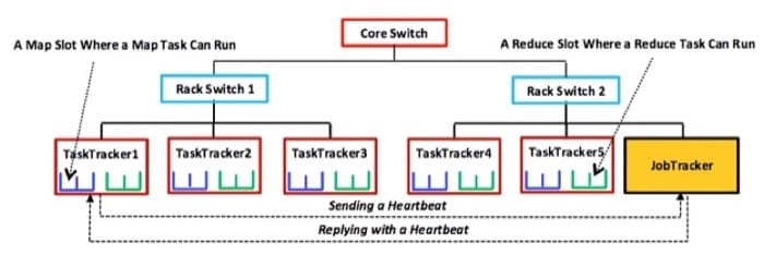
As Figure 5.18 shows, MapReduce uses a master-slave architecture. The master node is called JobTracker (JT), and each slave is called TaskTracker (TT). The JT and TTs communicate over the cluster network via a periodic heartbeat mechanism. By default, TTs send messages (heartbeats) to the JT every three seconds, and the JT replies6 with a new map or reduce task or with a different message. The JT uses these heartbeats to detect task failures (see the section Fault Tolerance). Each TT has, by default, two map slots and two reduce slots at which corresponding tasks can execute. This slot allocation determines the maximum number of map and reduce tasks (degree of task parallelism) that can run simultaneously in the TT.

Hadoop assumes a hierarchical, tree-style network topology with rack and core switches, as shown in Figure 5.18. TTs are spread over different racks and may reside in one or several data centers. Between any two TTs, communication bandwidth depends on their relative locations in the network topology. For instance, TTs on the same rack can interact with each other much faster than with off-rack counterparts. Measuring bandwidth between any two TTs is difficult in practice, so Hadoop employs a simple, distance-based approach, representing TT network positions as strings (e.g., TaskTracker5's location in Figure 5.18 is/CoreSwtich/RackSwitch1/TaskTracker5). Hadoop assumes a unit distance between any TT and its parent switch, so the total distance between any two TTs can be calculated by simply adding up the distances to their closest common ancestor. In our example, Total-Distance(/CoreSwitch/RackSwitch2/TaskTracker1, /CoreSwitch/RackSwitch2/JobTracker) = 4.

The JT does not reply to every heartbeat sent by a TT. TTs can send heartbeats just to indicate that they are still alive. If a TT includes in its heartbeat a request (e.g., a request for a map or a reduce task), the JT replies with a heartbeat that satisfies the TT's request (e.g., a map or a reduce task).

References

1. T. White (2011). "Hadoop: The Definitive Guide 2nd Edition." O'Reilly.
2. D. P. Bertsekas and J. N. Tsitsiklis (January 1, 1997). "Parallel and Distributed Computation: Numerical Methods." Athena Scientific, First Edition.

Job and Task Scheduling

Scheduling in MapReduce

MapReduce schedules work at both the job and task levels. Clients submit jobs, and the JobTracker (JT) partitions them into map and reduce tasks. Job scheduling (see the section Scheduling) determines which job should go next, and task scheduling orders tasks in a job. In Hadoop MapReduce, the JT schedules both jobs and tasks, although job schedulers are pluggable, that is, not part of the JT code. Task schedulers, on the other hand, are integrated in the JT code. The introduction of the pluggable job schedulers to the Hadoop framework is considered an evolution in cluster computing. Pluggable schedulers enable tailoring Hadoop for specific workloads and applications, which capability creates the opportunity for job schedulers optimized for the ever-increasing list of MapReduce applications. Furthermore, pluggable schedulers increase code readability and facilitate the experimentation and testing essential to research.

Hadoop MapReduce uses several alternate job schedulers, including a default first-in, first-out (FIFO) design and the Fair and Capacity schedulers. [13] FIFO suggests pulling jobs from a work queue in receipt order, oldest first, and launching them one after the other. Although such a strategy appears simple and easy to use, it suffers several drawbacks:

• FIFO scheduling does not support job preemption. Running jobs cannot be interrupted to allow waiting jobs to proceed and meet their performance objectives, such as avoiding job starvations and/or sharing resources effectively. As a result, simultaneous sharing of cluster resources is infeasible. As long as one job absorbs all cluster's resources (slots), no other can proceed. So the next queued job must wait until task slots become free, and the current job has no more tasks to execute. This limitation can easily lead to a fairness conflict, in which a long-running job blocks the whole cluster, starving all small jobs.
• The FIFO scheduler does not consider job priority or size, and a job's submission time alone completely determines its importance. Thus, jobs may wait in queue for extended periods, no matter how critical or time sensitive they are, and this limitation poses additional fairness and responsiveness issues.

To address the FIFO scheduler's shortcomings, Facebook developed a more sophisticated scheduler, called the Fair Scheduler, which is now part of the Apache Hadoop distribution. The Fair Scheduler represents cluster resources in terms of map and reduce slots and suggests a way to share clusters such that all jobs get, on average, an equal share of slots over time. The scheduler assumes a set of pools into which jobs are placed. Each pool is assigned a set of shares reflecting the map and reduce slots that its constituent jobs can occupy. The greater the number of shares a pool is assigned, the greater the number of map and reduce slots its jobs can use. Jobs in a pool can be scheduled using the FIFO scheduler or the Fair Scheduler itself. Jobs across pools are always scheduled using the Fair Scheduler.

When only a single job is submitted, the Fair Scheduler grants it all the cluster's available map and reduce slots. When new jobs are submitted, the scheduler assigns to them slots that become free. Assuming a uniform distribution of slots, each job thus gets roughly the same amount of CPU time. This strategy can obviously allow several jobs to run simultaneously on the same Hadoop cluster, "sharing in space" the cluster slots. This phrase implies that each job has exclusive access to a specific number of slots on the Hadoop cluster, an arrangement similar to sharing memory in operating systems (OSs), whereby the system allocates to each process an independent portion of the main memory. The result is that multiple processes can coexist(see the section Resource Sharing in Space and in Time for more details about sharing in space). Sharing in space, as offered by the fair scheduler, allows short jobs to finish in reasonable times while not starving long jobs. Jobs that require less time are able to run and finish while the jobs that require more time continue running. To minimize congestion due to sharing and finish work in a timely manner, the Fair Scheduler permits constraining the number of jobs that can be active at one time.

The Fair Scheduler can also accommodate job priorities by assigning to jobs weights that affect the fraction of total CPU time each can obtain. In addition, the scheduler can guarantee minimum shares to pools, thus ensuring that all jobs in a pool get sufficient map and reduce slots. Although a pool contains jobs, it gets at least its minimum share of resources, and when it becomes empty (no further jobs to schedule), the Fair Scheduler distributes its assigned slots uniformly across active pools. If a pool does not use all its guaranteed share, Fair can also spread excess map and reduce slots equally across other pools.

To meet every pool's guaranteed minimum share, the Fair Scheduler optionally supports preempting jobs in other pools. This procedure entails preempting some or all of the foreign map and reduce tasks in a rather brutal manner. Because Hadoop MapReduce does not yet support suspending running tasks (see the section on task elasticity in Scheduling ), the fair scheduler simply kills tasks in other pools that exceed their guaranteed minimum shares. Hadoop can tolerate losing tasks (see the sectionFault Tolerance), so this strategy does not cause the preempted jobs to fail, but it can affect efficiency because killed tasks must be reexecuted, thus wasting work. To minimize such redundant computation, the Fair Scheduler picks the most recently launched tasks from overallocated jobs as kill-candidates.

A third design, developed by Yahoo!, the Capacity Scheduler, shares some principles with the Fair Scheduler. As with Fair, the Capacity scheduler shares resources (slots) in space. However, it creates several queues, instead of pools, each with a configurable number (capacity) of map and reduce slots, and each queue can hold multiple jobs. All jobs in a queue can access the queue's allocated capacity. In a queue, scheduling occurs on a priority basis, with specific, configurable soft and hard limits, and the scheduler further adjusts priorities based on job submission times. When a slot becomes free, Capacity assigns it to the least-loaded queue and there chooses the oldest submitted job. Excess capacities among queues (unused slots) are temporarily assigned to other needy queues, even if the latter exceed their initially allocated capacities. If the original queue later experiences a demand for these reassigned slots, Capacity allows any tasks then running there to complete. Only when such tasks finish does the scheduler return the underlying slots back to their original queues/jobs (i.e., tasks are not killed). Although their reassigned slots perform "detached duty," the originating queues are delayed, but avoiding job preemption simplifies Capacity's design and eliminates wasted computation. Finally, like the Fair Scheduler, the Capacity Scheduler provides a minimum capacity guarantee to each queue. Specifically, each queue is assigned a guaranteed capacity so that the total cluster capacity is the sum of all queue capacities (no overcommitted capacity).

Scheduling a job under either FIFO, Fair, or Capacity implies scheduling all its constituent tasks. For the latter procedure, Hadoop MapReduce uses a pull strategy (see Symmetrical and Asymmetrical Architecture Models). That is, after scheduling a job, J, the JobTracker does not immediately push J’s Map and Reduce tasks to TaskTrackers, but rather waits for TTs to make appropriate requests via the heartbeat mechanism (see The Computation and Architectural Models). On receiving requests for map tasks, JT follows a basic scheduling principle that says, "moving computation toward data is cheaper than moving data toward computation." As a consequence, seeking to reduce network traffic, JT attempts to schedule map tasks in the vicinity of relevant HDFS input blocks. This goal is easy to accomplish because a map task's input is typically hosted at a single TT.

When scheduling reduce tasks, however, JT ignores that principle, mainly because a reduce task's input (partition(s)) usually comprises the output of many map tasks generated at multiple TTs. When a TT asks, JT assigns a reduce task, R, irrespective of TT's network distance locality from R's feeding TTs. This strategy makes Hadoop's reduce task scheduler locality unaware.

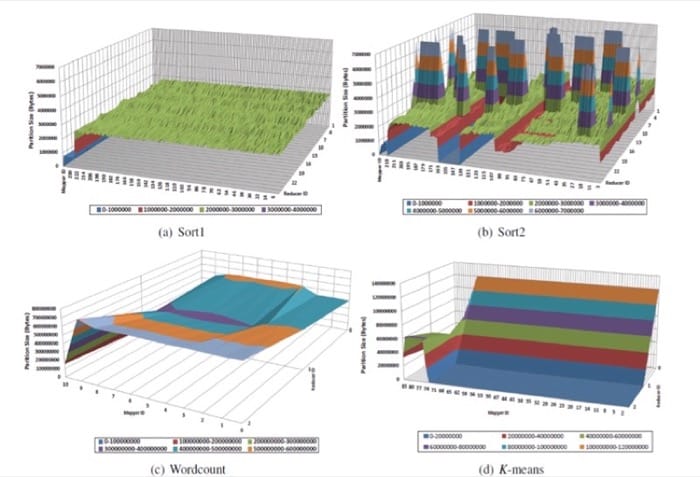
Hadoop's current reduce task scheduler is not only locality unaware but also partitioning-skew unaware (see the section The Data Structure and Flow). Partitioning skew refers to a significant variance in intermediate key frequencies and their distribution across different data nodes. Figure 5.20 demonstrates the partitioning skew phenomenon, showing partition sizes that each feeding map task delivers to each reduce task in two variants of the Sort benchmark, Sort1 and Sort2 (each with a different dataset), in WordCount and in k-Means.8 Partitioning skew causes shuffle skew, in which some reduce tasks receive more data than others. The shuffle skew problem can degrade performance because a job can get delayed while a reduce task fetches large input data, but the node at which a reduce task is scheduled can mitigate shuffle skew effects. In general, the reduce task scheduler's impact can extend to determining the network communication pattern, affecting the quantity of shuffled data, and influencing MapReduce job runtimes.

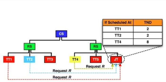
To make Hadoop MapReduce's reduce task scheduler more effective, it should address data locality and partitioning skew jointly. As a specific example, Figure 5.21 demonstrates a Hadoop cluster with two racks, each including three nodes. We assume a reduce task, R, with two feeding nodes, TT1 and TT2. The goal is to schedule R at a requesting TT, assuming TTs 1, 2, and, 4 poll JT for a reduce task. With the native Hadoop scheduler, JT can assign R to any of the requesting TTs. If R is assigned to TT4, TNDR will evaluate to 8. On the other hand, if R is assigned to TT1 or TT2,TNDR will be 2. As discussed earlier, a smaller TND should produce less network traffic and, accordingly, provide better performance.

References

1. S. Ibrahim, H. Jin, L. Lu, S. Wu, B. He, and L. Qi (Dec. 2010). "LEEN: Locality/Fairness-Aware Key Partitioning for MapReduce in the Cloud." CloudComm.
2. M. Hammoud and M. F. Sakr (2011). "Locality-Aware Reduce Task Scheduling for MapReduce." CloudCom.
3. M. Hammoud, M. S. Rehman, and M. F. Sakr (2012). "Center-of-Gravity Reduce Task Scheduling to Lower MapReduce Network Traffic." CLOUD.
4. Hadoop-scheduling. http://www.ibm.com/developerworks/linux/library/os-hadoop-scheduling/index.html.
5. Hadoop. http://hadoop.apache.org/docs/r1.1.2/fair_scheduler.html.
6. B. Thirumala Rao and L. S. S. Reddy (November 2011). "Survey on Improved Scheduling in Hadoop MapReduce in Cloud Environments." International Journal of Computer Applications.
7. M. Zaharia, D. Borthakur, J. S. Sarma, K. Elmeleegy, S. Shenker, and I. Stoica (April 2010). "Delay Scheduling: A Simple Technique for Achieving Locality and Fairness in Cluster Scheduling." EuroSys, pp. 265-278.
8. Mahout Homepage. http://mahout.apache.org/.
9. S. Huang, J. Huang, J. Dai, T. Xie, and B. Huang (2010). "The HiBench Benchmark Suite: Characterization of the MapReduce-Based Data Analysis." ICDEW.
10. P. C. Chen, Y. L. Su, J. B. Chang, and C. K. Shieh (2010). "Variable-Sized Map and Locality-Aware Reduce on Public-Resource Grids." GPC.
11. S. Seo, I. Jang, K. Woo, I. Kim, J. Kim, and S. Maeng (2009). "HPMR: Prefetching and Pre-Shuffling in Shared MapReduce Computation Environment." CLUSTER.
12. M. Isard, V. Prabhakaran, J. Currey, U. Wieder, K. Talwar, and A. Goldberg (2009). "Quincy: Fair Scheduling for Distributed Computing Clusters." SOSP.
13. A. C. Murthy, C. Douglas, M. Konar, O. O'Malley, S. Radia, S. Agarwal, and K. V. Vinod (2011). "Architecture of Next Generation Apache Hadoop MapReduce Framework." Apache Jira.

Fault Tolerance

Fault Tolerance in MapReduce

MapReduce's objective is to divide jobs into tasks that effectively exploit task parallelism and, consequently, complete jobs earlier. Although this approach is quite effective in theory, it exposes its own challenges in practice. For instance, it takes only one slow/faulty task to make the whole job consume significantly more time than expected. In reality, Hadoop MapReduce tasks fail and slow due to hardware degradation, software misconfiguration, heterogeneity, and/or data locality, to mention a few problems. Tolerating faulty and slow tasks in clouds is not easy. In particular, when the volumes of data flowing through an I/O system are as big as those processed by Hadoop, the chance of data pieces getting corrupted increases. Furthermore, when tasks and nodes operate in the thousands and beyond (typical for Hadoop), chances of failure increase.

Hadoop MapReduce applies two mechanisms to tolerate faults, data redundancy, and task resiliency. Data redundancy is applied at the storage layer. Specifically, HDFS reliability retains HDFS blocks by maintaining multiple replicas per block (by default, three replicas) at physically separate machines (see the section The Hadoop Distributed File System (HDFS) in Unit 4). Clearly, this enables MapReduce to tolerate corrupted blocks and faulty nodes easily. If a block is lost due to a hardware or software failure, another replica at a different node can always be located and read in a way totally transparent to user jobs. HDFS computes checksums using a cyclic redundancy check (CRC-32) for all data written to it and, by default, verifies checksums when reading data from it. When a block error is detected or a node goes down, HDFS transparently brings back the replication factor to its default level of three.

Although it is possible that all the HDFS blocks of a job's dataset are error free, the job's tasks may still run slowly or simply fail. Clearly, a task slowdown or failure a can lead to slowing an entire job or causing it to fail. To avoid such consequences and to achieve resiliency, Hadoop MapReduce allows replicating tasks and monitors tasks to detect and treat slow/faulty ones. To detect slow/faulty tasks, Hadoop MapReduce depends on the heartbeat mechanism (see the section The Data Structure and Flow). The JobTracker (JT) runs an expiry thread that checks each TaskTracker's (TT) heartbeats and decides whether the TT's tasks are dead or alive. If the expiry thread does not receive heartbeats confirming a task's health within 10 minutes (by default), the task is deemed dead. Otherwise, the task is marked alive.

Alive tasks can be slow ("stragglers" in Hadoop's parlance) or not slow. To measure slowness, JT estimates task progress using a per-task score between 0 and 1. Map and reduce scores are computed differently. For a map task, the progress score is a function of the input HDFS block read so far. For a reduce task, the progress score is more involved. Hadoop MapReduce assumes that each of the reduce stages (shuffle, merge and sort, and reduce) accounts for one-third of a reduce task's score, and, for each stage, the score is the fraction of data processed so far. For instance, a reduce task that is halfway through the shuffle stage will have a progress score of 1/3 * 1/2 = 1/6. On the other hand, a reduce task that is halfway through the merge and sort stage will have a progress score of 1/3 + (1/2 * 1/3) = 1/2. Finally, a reduce task that is halfway through the reduce stage will have a progress score of 1/3 + 1/3 + (1/3 * 1/2) = 5/6.

When it detects a slow task, JT runs a corresponding backup (speculative) task simultaneously. Hadoop allows one speculative task per original slow task, and the two compete. Whichever version completes first is committed, and the other is killed. This task-resilience tactic is known in Hadoop MapReduce as speculative execution and is activated by default, although it can be enabled or disabled independently for map and reduce tasks, on a cluster-wide or per-job basis.

Hadoop MapReduce computes the average progress score across all tasks in each task category (e.g., all map tasks). In a category, any task scoring less than 80% of the mean (called the 20% progress-difference threshold) is marked a straggler, and, as long as all original map and reduce tasks are already scheduled,9 JT launches an equivalent,speculative task. All stragglers are treated as equally slow, and ties between them are broken by data locality. More precisely, if a map slot becomes free at a particular TT, and two map stragglers are detected, the one that uses an HDFS block stored at TT will be selected for speculative execution. If the two stragglers will both need HDFS blocks stored at TT, one can be chosen randomly. Dead tasks always get highest priority and speculative tasks get the lowest. In particular, when the JT receives a TT heartbeat that includes a map or a reduce task request, JT replies with a task in the following order: (1) a task that compensates for a dead/stopped task, (2) an original, not yet scheduled task, or (3) a speculative task.

Hadoop MapReduce's task-resiliency approach works well in homogeneous environments but falters in heterogeneous ones for several reasons:

• Heterogeneity can result from resource contention in virtualized clouds (see the section Heterogeneity), in which the congestion may be only transient. In such cases, JT may launch too many speculative tasks for originals that appear slow at the moment but are shortly thereafter identified as not-slow. Speculative tasks take resources away from originals, and excessive speculative executions can slow the entire cluster, especially if the network is overloaded with a great deal of unnecessary shuffling traffic.
• Hadoop MapReduce also launches speculative tasks at TTs without considering how their current loads/speeds compare with those of TTs hosting the original tasks. Potentially, JT could schedule a speculative task at a slow TT that subsequently becomes slower than even the corresponding original task.
• Because the Hadoop scheduler uses data locality to break ties among map stragglers, the wrong stragglers can be selected for speculation. If JT detects two stragglers, S1 and S2, of which S1's score is 70% of the average and S2's is 20%, and if a TT hosting S1's input block becomes idle, S1 could be speculated before S2.
• The 20% progress-difference threshold implies that tasks scoring over 80% of the average will never be speculated, despite necessity or potential efficiency gains.
• Finally, Hadoop MapReduce divides the reduce phase score equally across its three constituent stages. This compromise is unrealistic in a typical MapReduce job, in which the shuffle stage is usually the slowest due to involving all pairs communicating over the network. In actuality, it is highly likely that after the shuffle stage, MapReduce jobs quickly finish the merge and sort and the reduce stages. Therefore, soon after the first few reduce tasks finish their shuffle stages, their progress scores will jump from 1/3 to 1. This will significantly increase the overall average score and potentially degrade the accuracy of speculation. In fact, as soon as 30% of reduce tasks commit, the average score becomes 0.3 * 1 + 0.7 * 1/3 = 53%. Subsequently, all reduce tasks that are still in the shuffle stage will be 20% behind the average score. As a result, an arbitrary set of false stragglers will be speculated, filling up reduce slots quickly and possibly overwhelming the cloud network with unnecessary traffic.

Clearly, Hadoop MapReduce's standard speculative execution approach suffers from serious shortcomings. For this reason, Facebook disables speculative execution for reduce tasks, and Yahoo! likewise disables speculative execution altogether, although only for certain jobs. To address the underlying problem, Zahria and associates propose a greedy strategy called longest approximate time to end (LATE), which suggests that only those tasks expected to finish farthest in the future can be speculated. LATE provides the greatest opportunity for speculative tasks to overtake originals and, accordingly, should tend to decrease job response times. However, the challenge lies in identifying appropriate candidate tasks. To do so, LATE proposes computing the progress rate of each task as progress score/T, where T is the time the task has taken so far, and then predicting the task's time to completion as (1-progress score)/progress rate. In addition, LATE promotes scheduling speculative tasks at only fast TTs (those above a certain threshold). Also, to account for the fact that speculation consumes resources, LATE specifies a cap on the number of speculative tasks that can be launched at once. Last, LATE overlooks data locality upon scheduling speculative map tasks, assuming that most original map tasks still run with local input HDFS blocks and commit successfully. Experimentation results show that LATE can improve Hadoop response times two-fold on Amazon Elastic Compute Cloud (EC2), a heterogeneous cloud environment.

References

1. M. Zaharia, A. Konwinski, A. Joseph, R. Katz, and I. Stoica (2008). "Improving MapReduce Performance in Heterogeneous Environments." OSDI.
2. T. White (2011). "Hadoop: The Definitive Guide, 2nd Edition." O'Reilly.
3. Z. Guo and G. Fox (2012). "Improving MapReduce Performance in Heterogeneous Network Environments and Resource Utilization." In Proceedings of the 2012 12th IEEE/ACM International Symposium on Cluster, Cloud and Grid Computing.

YARN The New Hadoop MapReduce

Hadoop 2.0 and YARN

Hadoop has undergone a major overhaul to address several inherent technical deficiencies, including the reliability and availability of the JobTracker (JT) and the static resource (map and reduce slots) allocation at TaskTrackers (TTs), to mention a few. The redesigned framework addresses such problems in the JT, Hadoop's master node and, therefore, a single point of failure (SPOF). Another major objective for the new Hadoop is to support, in addition to MapReduce, other distributed analytics engines. This allows for increased utilization of Hadoop clusters and eliminates the need for a large cluster to be deployed for each framework. For Hadoop, the result is a new version named Yet Another Resource Negotiator (YARN). We next introduce YARN and point out how it differs from the previous Hadoop MapReduce, which we call MapReduce 1.0.

YARN is the second generation Hadoop (version 2.0 and higher). The main advantage of YARN from the previous generation of Hadoop is that the resource allocation is no longer fixed, and YARN is not bound to any single programming framework. This allows YARN to function as an independent cluster scheduler, which is capable of scheduling different workloads and applications. YARN is a two-level scheduler, the responsibility of the Job Tracker in Hadoop v1 in YARN is separated into resource allocation and task management, which enables YARN clusters to easily scale up.

Architecture and Workflow

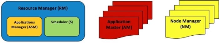
The fundamental change pursued in redesigning MapReduce 1.0 was segregating JT functionalities into multiple, independent daemons, illustrated in Figure 5.22. YARN still employs a master-slave topology but adds several enhancements:

1. To support other distributed analytics engines in addition to MapReduce, the resource management module has been entirely detached from the JT and defined as a separate entity, the ResourceManager (RM). RM has been further sliced into two main components, the Scheduler (S) and the ApplicationsManager (AsM).
2. Instead of using a single master, JT, for all applications, YARN appoints one master per application, an ApplicationMaster (AM). AMs can be distributed across cluster nodes to avoid application SPOFs and potential performance degradations.
3. TTs have remained effectively unchanged but are now called NodeManagers (NMs).

Components of YARN

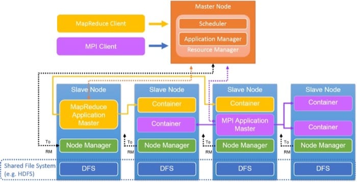
A per-cluster Resource Manager (RM) resides in the master node (Figure 5.23). The RM accepts application/job submissions by a client, allocates resources to jobs, monitors the cluster state and manages the access to resources. The RM has two components: the Scheduler (S), which schedules job, and the Applications Manager, which creates, manages, monitors, restarts and kills jobs.

The RM is the central authority, it arbitrates resource allocations among various competing applications/jobs. The RM dynamically allocates resources as leases to applications in the form of containers. Containers are a logical representation of resources in the form of amount of memory or number of CPUs. Currently, the RM handles memory capacities and CPU resources but does not yet support disk, or network resources. The RM interacts with Node Managers (NMs) to assemble a global view of the cluster and to enforce resource assignments. The RM tracks resource usage and node liveness through a heartbeat mechanism.

The Scheduler is a part of the RM and builds a global plan for cluster resources, serves application resource needs, and schedules jobs using strategies such as Capacity or Fair scheduling. The Applications Manager, another part of RM, accepts submitted jobs, negotiates with the Scheduler to initialize resources, a container, to run a job’s Application Master (AM), and provides services for tolerating/restarting the AMs when failures occur.

The Application Master (AM) coordinates the application’s (or job’s) execution in a YARN cluster. Each job, be it a MapReduce job, MPI job, or Spark job, has a dedicated AM in the YARN cluster. The AM runs in a common container as other tasks do. The AM is responsible for getting containers and allocating its tasks on to them. It computes the set of resources it needs based on the tasks it has to run and sends a request to the RM. Once the resources are allocated it runs the tasks on those containers and once they complete it gives them back to the RM. Below we explain this process in more detail.

As the AM runs in a container, it sends periodic heartbeats to the RM to update its liveness and to update its resource demands. The AM calculates the resources demands of its job and makes a request for containers along with preferences and constraints within its periodic heartbeat message to the RM. In turn, the RM dynamically responds to the heartbeat in the form of container leases (provided as tokens). The AM uses the tokens when contacting the corresponding NMs to start a job’s tasks. The AM keeps track of the status of its running tasks through an umbilical mechanism. During a job’s execution, the RM is blind to the AM’s scheduling. For a MapReduce job, the AM is like the JobTracker in Hadoop version 1.0.

The Node Manager (NM) resides on each node, a single NM per YARN cluster node. The NMs authenticate container leases and monitor resource utilization. NMs contact the RM through heartbeats and kill containers as directed by the RM or AM. A container represents a lease for an allocated resource in the cluster. A lease is a logical bundle of resources bound to a node. The RM is the sole authority to allocate any container to jobs. Every allocated container has a unique ContainerId, which is globally unique. Each container has a number of non-static attributes: CPU, memory, disk BW, network BW. Containers can be compared to MapReduce slots in Hadoop version 1.0. A container is killed shortly after the task running in it finishes, and RM revokes the resources and makes use of it later.

When requiring compute resources, the AM presents to the RM Scheduler a series of container requests. The protocol understood by the Scheduler is <priority, (host, rack, *), resources, #containers>. The RM Scheduler assigns or allocates containers in the same format. A snapshot from the RM log, shows how the RM allocates a container (Figure 5.24):

Job and Task Scheduling

YARN is a two-level scheduler, the RM schedules jobs and the AM schedules its tasks on the containers it gets allocated by the RM. The Scheduler, which is responsible for job scheduling in the RM employs different scheduling strategies:

• FIFO Scheduler: is a basic and simple scheduler which has a single first in first out queue and schedules the container requests based on that. Typically, a job can exclusively occupy resources within the cluster while running. Though each job can be offered large resources, this creates problems such as starving other jobs or not sharing the available resources fairly. The FIFO scheduler allows job priorities to be set, hence, the job with the highest priority is selected as the next job to run. However, since the FIFO scheduler does not support preemption the problem of job starvation still exists. A high-priority job can be blocked by a long-running but low-priority job.
• Capacity Scheduler: assumes that Hadoop jobs are running on a shared, multi-tenant cluster and maximizes the throughput and utilization of the cluster. The Capacity Scheduler guarantees to users that are sharing a large cluster to get capacity guarantees. The Capacity Scheduler organizes jobs in queues. Typically, the queues are setup by administrators based on how the YARN cluster will be partitioned and utilized by different groups of users (group 1, queue 1 gets 50% of the cluster). The Capacity Scheduler offers a set of limits to make sure a single job or queue cannot consume disproportionate amount of resources in the cluster.
• Fair Scheduler: focuses on running different YARN jobs fairly, providing jobs with an equal share of resources over time. By default, a scheduling decision made by the Fair Scheduler is based only on memory. However, the Fair Scheduler is configurable, and it can schedule with both memory and CPU. The Fair Scheduler ensures some short jobs to finish in a reasonable amount of time without starving large or time-consuming jobs. It is also a desirable scheduler for multiple users sharing the same cluster. Besides allocating resources equally, the Fair Scheduler can also schedule jobs with different priorities. Priorities, set by users, can be used to determine how many resources each job should be assigned.
• Your Scheduler: users can plug in their own job scheduler.

The strategies of scheduling can be configured in the file yarn-site.xml. There are also many properties that can be set in yarn-site.xml to tune the operational parameters of the schedulers mentioned above.

After a job is allocated resources (containers), the AM is in charge of scheduling a job’s tasks on these containers. The AM schedules tasks in the same way the JobTracker does in Hadoop version 1.0. Moreover, the AM also takes the responsibility of monitoring the status of tasks, which is done by TaskTracker in Hadoop version 1.0.

Fault Tolerance in YARN

The Resource Manager (RM) is a single point of failure (SPOF) of a YARN cluster. The Resource Manager checkpoints its state to persistent storage periodically. If the RM fails, it can be restarted from one of the checkpoints. All running AMs are then killed and restarted and the applications and tasks that are pending from the checkpoint state can be scheduled and executed.

Any AM may fail. The RM will notice an AM’s failure to send a heartbeat, and will restart the AM. However, the AM has to resync with all running containers to ensure the job finishes smoothly.

The NM failures can also be detected by the RM. When a NM fails, all containers on this node will be killed and the failure will be reported to all running AMs. The AMs are responsible for acquiring new resources in the form of containers from the RM to run the killed tasks, and no more containers will be assigned on the failed node in the cluster until it recovers and reports back to the RM.

An example: WordCount

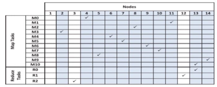
Here we present an example of running WordCount on a YARN cluster consisting of 1 master node and 4 slave nodes. We employ the m1.large instance (2 vCPU, 6.5ECU, 7.5GB Memory) offered by Amazon Web Service (AWS). The input data is partitioned as 39 plain text files on the distributed file system, which are 2.32 GB in total. The number of map tasks is computed to be 39, and we manually configure the number of reduce tasks in the job configuration file to be 7.

We use snapshots to detail the execution process of this job on YARN:

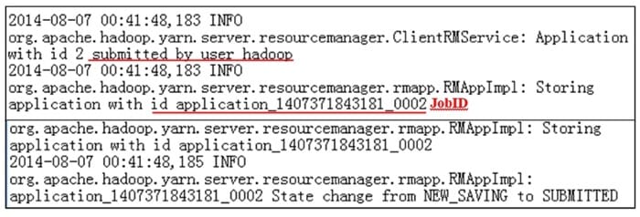
1. The client starts to run the WordCount job.
2. The RM assigns a jobID for this WordCount job.
3. Information of this WordCount job is saved or copied to HDFS.
4. The WordCount job is submitted to the RM (Figure 5.27).
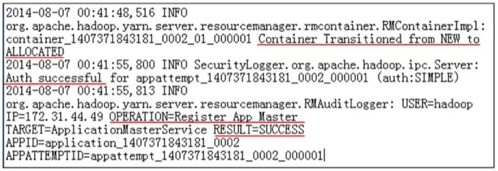
5. The RM communicates with the NM to allocate a container for the AM.
6. The NM authenticates the container lease from the RM.
7. The RM succeeds in launching the AM for the WordCount job (Figure 5.28).
8. The AM starts running, and it computes resources it needs to finish the WordCount job: 39 map tasks and 7 reduce tasks.
9. The RM receives requests from the AM and allocates resources in the form of containers.
10. The AM sends the lease to NMs and a bunch of containers get running.
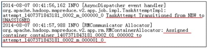
11. The AM starts map task attempts, ready to run in containers. In our case, the AM, in the first place, starts 12 map task attempts because there aren’t enough resources for other container on our 4-node cluster.
12. The AM then assigns containers to map task attempts based on its knowledge of data locality (Figure 5.29).
13. The map tasks start running. While running, the AM keeps track of the status of each task attempt through a heartbeat mechanism. • At some point, a map task finishes executing in a container and the AM is informed.
14. This container is then cleaned by the AM. Compute resources are retrieved and a new container will be started by the NM through the same process mentioned above. The AM will assign new map or reduce task attempt to the new container. Only one task can be run in one container.
15. Because of the early shuffle, when several map tasks finish (at least 5% by default), the AM will assign a reduce task attempt to an available container. A reduce phase consists of the shuffle, merge and sort, and the execution of the reduce function. Only after the output bytes of the reduce task are written to HDFS can a reduce task finish.
16. The AM manages all the map and reduce tasks, it waits for their completion. Once the last reduce task finishes, the whole job will be marked FINISHED.
17. The AM communicates with the NMs to clean up all remaining containers.
18. The AM will notify the RM that the job is completed.
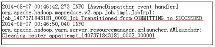
19. The RM cleans up the AM. The whole WordCount job ends (Figure 5.30).

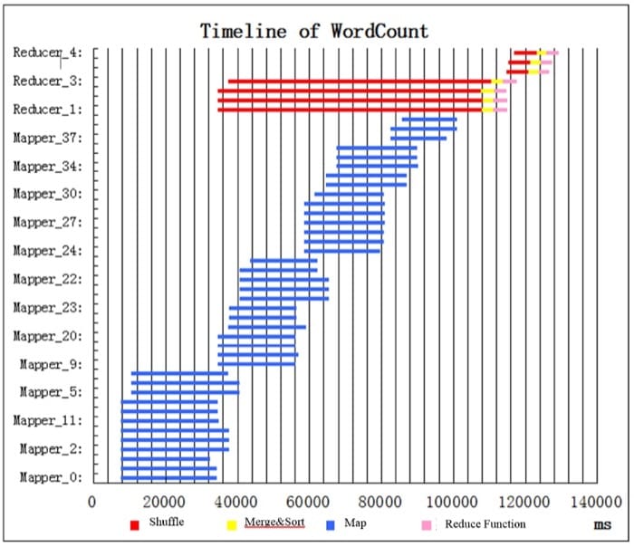
A timeline of tasks for an example WordCount job:

Shortly after the job starts, 12 map tasks (blue bars) start running (Figure 5.31). No more map task can be run because no more resources (containers) are available in the cluster to start another map task. We refer to several map tasks running in parallel as a wave, so, we have 12 map tasks in the first wave. After a period of time, some of the map tasks finish. Due to the early shuffle mechanism (by default when 5% of the map tasks finish, reduce tasks are scheduled and the begin to shuffle). In this example, there are enough resources for four reduce tasks to start. Each reduce task has 3 sequential subphases: shuffle(red), merge&sort(yellow), reduce function(pink). While the 4 reduce tasks are performing an early shuffle, the second wave of map tasks begins to run. When the last map task completes, the whole map phase ends. Afterwards, themerge&sort and reduce functions can run. Afterwards, there are enough containers to run 3 more reduce tasks. The job finishes shortly after the last reduce task ends.

References

1. Big-Data Analytics Predictions for 2011. http://tdwi.org/articles/2011/03/16/big-data-analytics-predictions.aspx/.
2. T. White (2012). "Hadoop: The Definitive Guide, 3nd Edition." O'Reilly.
3. A. C. Murthy, C. Douglas, M. Konar, O. O'Malley, S. Radia, S. Agarwal, and K. V. Vinod (2011). "Architecture of Next Generation Apache Hadoop MapReduce Framework." Apache Jira.
4. Vavilapalli, Vinod Kumar and Murthy, Arun C and Douglas, Chris and Agarwal, Sharad and Konar, Mahadev and Evans, Robert and Graves, Thomas and Lowe, Jason and Shah, Hitesh and Seth, Siddharth and others (2013). "Apache hadoop yarn: Yet another resource negotiator." Proceedings of the 4th annual Symposium on Cloud Computing.

Summary

• MapReduce is a data-parallel framework for processing big-data applications on large clusters. Hadoop is an open-source implementation of MapReduce.
• MapReduce programs typically have a map and a reduce phase. MapReduce also uses an underlying distributed file system, which, in the case of Hadoop, is HDFS.
• In the map phase, the input data is divided into splits and processed independently by map tasks. The output of the map tasks is sorted and shuffled into partitions that are copied to reduce tasks. Reduce tasks process the partitions and produce the final output.
• Data in MapReduce is always formatted as a set of key-value pairs. Keys in MapReduce are used for shuffling data in between the map and reduce phases.
• Examples of MapReduce programs discussed in this module include WordCount, Sort, and Sobel edge detection.
• A MapReduce cluster comprises a JobTracker (which is the master node) and TaskTrackers (slave nodes).
• JobTrackers assign tasks to TaskTrackers using a pull strategy and monitor TaskTrackers and their progress in executing tasks through a heartbeat mechanism.
• Hadoop supports multiple job schedulers, including FIFO, Fair, and Capacity, among others.
• The FIFO scheduler is the default scheduler which executes jobs in the order they arrive at the cluster. It does not consider job priority or size, and a small job that might take minutes to run will have to wait for a long-running job that is in the queue to complete first.
• The Fair Scheduler allows cluster resources to be shared among multiple jobs such that all jobs get an equal share of the cluster slots over time.
• The Capacity Scheduler is a more complex version of the Fair Scheduler that creates multiple job queues and schedules jobs on a priority basis.
• Map tasks in Hadoop are executed on nodes that are closest to the split that needs to be processed. Reduce tasks, however, are processed on any node by default, without paying attention to locality.
• Data redundancy in Hadoop is provided by HDFS through block replication.
• Tasks resiliency in Hadoop is provided by speculative execution, whereby task progress is continually monitored by the JobTracker and slow/stuck tasks are reexecuted on another node as a speculative task.
• Hadoop 2.0 provides a new resource manager called YARN, which provides several enhancements over MapReduce 1.0.