云计算 阅读材料 14 Cloud Storage

We now move on to the next part of the course, namely Cloud Storage. Storage is an important aspect of cloud computing and has seen a lot of innovation in the last decade or so. In fact, Amazon’s first public cloud service was the Simple Storage Service (S3).

---

We will begin with a description of the types of and characteristics of data. We will then move to typical applications and their requirements on storage systems.

We will then explore storage devices and recap the various types of devices that are currently used in storage systems. Next, we visit the various abstractions that are used to organize data - either as blocks on disk, files within a file system or as objects in a database. We will then explore each of those abstractions in detail.

The first abstraction we will dive into is file systems. We will discuss the different types of file systems as well as their design considerations. We will then explore databases, consider the various design choices made when creating database systems and discuss the three main types of databases that are popular today: Relational, NoSQL and NewSQL databases. We will finally end this unit with a discussion on a class of cloud specific storage systems, namely object storage as a cloud service.

Data

Data is simply a collection of raw facts and figures. Applications are responsible for generating, storing, analyzing and consuming data, or some combination thereof.

The nature and properties of data typically influence the design and implementation of storage systems. Some of the properties include volume, content, and the frequency of access of data. As an example, Facebook [2] recently studied the access patterns of image and video content posted by its users to find that the access rate exponentially decreases as time passes. They used these findings to design and implement a storage system specific to their needs. In video 4.1, we will look at the various properties of data that influence the design of storage systems.

Video 4.1: Characterizing Data

Structure of Data

Data can be categorized using its dynamicity and structure. Specifically, data can be broadly segmented into one of the four quadrants in Figure 4.1. One categorization represents the structure of the data, which is considered as either structured or unstructured.

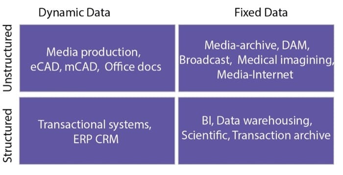
Structured data have a predefined data model that organizes the data in a form that is relatively easy to process, store, retrieve, and manage. Structured data are usually small data that naturally fit in tabular form and hence can easily be stored in traditional databases (e.g., relational databases). An example of structured data is customers' contact information that is stored in tables in a customer relationship management (CRM) database. These data fit in a fairly rigid model (called schema in relational databases), which can be quickly stored, accessed, and manipulated.

Unstructured data, on the other hand, may not necessarily have a predefined, rigid organizational model. Unstructured data may be larger and may not fit naturally in tabular form, making the data unsuitable for storage in a relational database. Thus, unstructured data may be relatively difficult to organize in a form that is simple to process, store, retrieve, and manage. Examples of unstructured data are flat binary files containing text, video, or audio information. It is important to note that unstructured data is not necessarily devoid of structure; a document, video, or audio file may have a file encoding structure or metadata with which it is associated. Hence, data with some form of structure may still be characterized as unstructured if their structure is not helpful to the processing task for which the data are needed. To illustrate, a large cache of text documents (which are unstructured) is difficult to index and search when compared to a relational database containing customer information (which is structured). For the purposes of this course, unstructured data can be defined as data that do not fit naturally in a relational database. In addition, some data may be treated as unstructured (not stored in a database) because they will be accessed using unpredictable access patterns; traditional database optimizations are pointless for such data.

There is a type of data that lies between structured and unstructured, referred to as semi-structured data. Semi-structured data does not conform with the formal structure of data models associated with relational databases or other forms of data tables, but nonetheless contains tags or other markers to separate semantic elements and enforce hierarchies of records and fields within the data. Data that is described using markup languages, for example web pages, clickstream data, web objects are examples of semi-structured data. XML and JSON are classic examples of representations of semi-structured data as they inline data with tags that describe the data as well.

Dynamicity of Data

Another characterization is the dynamicity of the data, which is an indication of how often the data changes. Dynamic data, such as Microsoft Office documents and transactional entries in a financial database, change relatively frequently, whereas fixed data, once created, may not be altered. Examples of fixed data include medical imaging data from MRI and CT scans and broadcast video footage that is archived in a video library.

Segmenting data into one of these quadrants helps in designing and developing a storage solution for the data. Structured data are typically processed using relational databases in which the data can be accessed, managed, and manipulated using precise commands (typically issued in a query language such as SQL). Unstructured data may be stored in flat files in a file system or may be further organized using a NoSQL database (more on NoSQL later in the module).

The structure and dynamicity of data provide guidance on how a storage system can be architected. Large amounts of data that are relatively static can be stored on disk arrays if they are read frequently. Storage systems designed with multi-tiered caching architecture (such as multi-tiered with caching) improve the performance of read operations on such data.

Certain types of file systems, such as earlier versions of the Hadoop Distributed File System (HDFS), are designed for relatively static data. They allow a file to be written only once, and the file cannot be modified after it is written. Static data, such as drive images and snapshots for backups, can be archived on relatively inexpensive offline storage systems if they do not need to be accessed frequently.

In summary, the nature of data used by an application must be considered before its appropriate storage architecture is chosen.

Granularity and Volume of Data

In addition to the type of data, the volume of data that needs to be stored and processed for a particular application must be considered. The volume of data is characterized along two dimensions, the overall size of data (total volume), versus the size of a useful segment of the data (the granularity of data). As an example, consider the case of a photo sharing website that has millions of users posting tens to hundreds of photos to the website. The total size of the data may be tens or hundreds of terabytes or even petabytes, but the average photo may be a few megabytes. Contrast this to a website like youtube, where the total size of all the videos in youtube is many petabytes, and the size of an video can range from a few hundred megabytes to even gigabytes in size.

In this regard, we touch on an often-used term to describe large volumes of data: big data. There are many definitions of big data, but one popular description summarizes it as data is too big to be handled using conventional techniques.

The rapidly expanding information and communications technology (ICT) that is permeating all aspects of modern life has led to a massive explosion of data over the last few decades. Major advances in the connectivity and digitization of information has led to increasing amounts of data being created on a daily basis. These data are diverse, ranging from images and videos from mobile phones being uploaded to websites such as Facebook and YouTube, to 24/7 digital TV broadcasts, to surveillance footage from hundreds of thousands of security cameras, to large scientific experiments such as the Large Hadron Collider—all of which produce many terabytes of data every day. International Data Corporation's (IDC) latest Digital Universe Study predicts a 300-fold increase in the amount of data created globally from 130 exabytes (1028) in 2012 to 30,000 exabytes in 2020 (Figure 4.2).

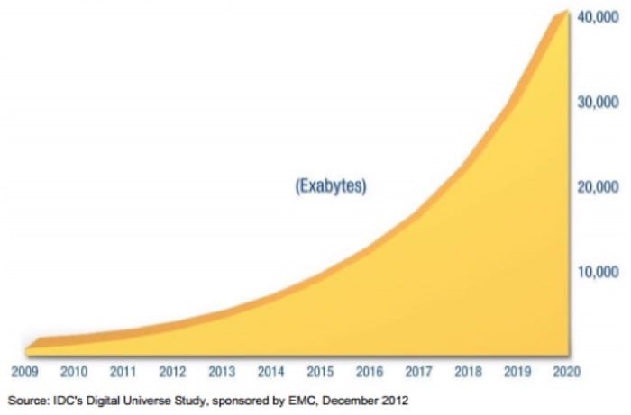
Organizations are trying to leverage or, in fact, cope with the massive amounts of data that are growing at ever-increasing rates. Google, Yahoo!, and Facebook have gone from processing gigabytes and terabytes to the petabyte range, which puts immense pressure on their computing infrastructures that need to be available 24/7 and must scale seamlessly as the amount of data produced rises exponentially. These are the challenges to which present and future storage technologies must respond.

References

1. John Gantz and David Reinsel (2012). "The Digital Universe in 2020." IDC White paper.
2. Subramanian Muralidhar, Wyatt Lloyd, Sabyasachi Roy, Cory Hill, Ernest Lin, Weiwen Liu, Satadru Pan, Shiva Shankar, Viswanath Sivakumar, Linpeng Tang and Sanjeev Kumar (2014). "f4: Facebook's Warm BLOB Storage System." 11th USENIX Symposium on Operating Systems Design and Implementation (OSDI 14). USENIX Association. 383-398 Pages.
3. Thomas Rivera (2012). "The Evolution of File Systems." SNIA Tutorial.

Applications and Requirements

Applications can deal with data in many ways. Some applications serve to be storage and retrieval systems of data. They may archive data for a variety of reasons. Backup software archives user data in a snapshot fashion, allowing the user to restore the state their computer and files in the event of a hardware failure or accidental deletion. Large websites such as archive.org crawl popular websites and preserve a snapshot allowing users to view the previous versions. A retailer may want to store information regarding every individual transaction for accounting and tax purposes.

Other applications retrieve data to enable decision making. One example of this is business intelligence systems. A business intelligence system can process millions of transactions and infer sales trends. This information could be used to enable inventory and marketing decisions to be made by the retailer.

Applications can also extract knowledge for analysis. As an example, Google [1] recently discovered that search trends of certain keywords is highly correlated with physician visits for influenza-like visits. This enables Google to publish information about flu trends that is updated daily.

Data can also enable a service. Almost any type of dynamic web service which responds to user requests is an example of this. Specific instances include: mapping and navigation software. By collecting information about road networks and addresses, a system (such as Google Maps) can respond to direction-related queries.

Application Requirements

Different applications have different requirements of storage systems. Netflix, for example needs to serve high-bandwidth video to millions of users across the countries in which they operate in. Google search, on the other hand, must analyse a query and retrieve accurate results for that query within a very short period of time. In this section, we will look briefly at the various requirements imposed by applications on storage systems:

1. Capacity: Storage systems must be able to handle the capacity requirements for an application. A storage system should be able to handle the entire volume of data that is required by the application, and must also be scalable in some form to meet the near and future-term requirements of the application.
2. Performance: Storage systems should be able to handle application expectations of performance. This can be broadly broken down into the following requirements:
   • Latency: The system should respond to requests within a certain expected time frame. In web-scale systems this requirement is quite important as it directly relates to the user's experience
   • Bandwidth: The system should be able to move data at a certain rate. For applications that rely on continuous feeds of data (such as video), this is a crucial metric.
3. Access Patterns: The particular patterns in which an application accesses data can be used to design and implement efficient storage systems. Specifically the following patterns are of interest to storage systems designers:
   • Granularity of Access: The granularity of access refers to the smallest amount of data retrieved in a typical operation. This can range from a few bytes to multiple megabytes, depending on the type of application.
   • Frequency of Access: Frequency of access refers to how often data is accessed from the system. If there are certain elements that are constantly accessed, they provide avenues for optimization through techniques such as caching.
   • Locality of Access: Refers to spatial and temporal locality. An example of locality is how distant data elements are when they are retrieved for the application. Locality can be considered both at the micro level (how far apart is the stride in an array index during a matrix multiplication), or even at the macro level (which data center worldwide should respond to this particular user's request)?
4. Durability: This refers to the applications expectations of how the data on the system needs to be persisted.
5. Fault Tolerance: Fault tolerance is a generic term that denotes several attributes of a system. They can be described in terms of the following requirements:
   • Reliability: If a particular data item is reported as written by a system, can it be always be retrieved back from the system?
   • Availability: Is there a particular period of time where the system does not respond to requests? How often does this happen? Is my application affected by this, and what can be done to minimize the impact of this downtime?
   • Accuracy: How accurate are the results returned by the system? This may seem like a trivial question for a simple system that consists of only a single data store, but if a system is distributed with multiple copies of the same data, this may pose to be a very significant issue. Some applications can deal with data that is a bit stale, but others require an accurate answer every single time.
6. Security: How secure does the data need to be when it is stored and accessed by the application? Is it protected against accidental or malicious access and/or modification and deletion? What kind of access restrictions can be imposed on users and applications that access this system?
7. Provenance: The process by which one can trace and record the origin of data as well as its movement between storage systems. For an application, does the functionality of being able to track all this information necessary? For certain applications dealing with sensitive and/or confidential data, it is a requirement.

These requirements dictate the design of applications. Applications that require large capacity or need scalability in the near or long term need to be architected accordingly. As you will see in this Unit, storage systems that deal with large volumes of data are typically too slow or expensive to be contained within a monolithic system, these are typically distributed over multiple machines.

Strict performance requirements are usually translated into design choices involving caching or replication. Such systems are designed using the access patterns to determine optimal strategies for performance improvement. For applications that are serving clients over the internet, multiple data centers may be involved to provide faster performance and a better user experience by redirecting users to the closest available server that has the required data.

In order to use certain replication or caching techniques, the applicaiton must decide on what level or accuracy or freshness it needs of the data retrieved from the system. Certain applications may be ok it they recieve stale data, but others require the most accurate and up-to-date data. This in turn affects the level of consistency that the storage system must provide to the application.

References

1. Ginsberg, Jeremy and Mohebbi, Matthew H and Patel, Rajan S and Brammer, Lynnette and Smolinski, Mark S and Brilliant, Larry (2009). "Detecting influenza epidemics using search engine query data." Nature.

Storage Devices

We shall now dive into the actual devices used to store and persist data in Video 4.2. This video should serve to be a refresher on various types of storage technologies that are available, with their relative cost-performance tradeoffs.

Video 4.2: Storage Devices

Memory Hierarchy

As a quick recap, the memory hierarchy is illustrated in Figure 4.3 below. The fastest (and most expensive) storage space in a modern computer is the on-chip registers, which consist of about sixteen 8 byte registers per core. These can be accessed within a single clock cycle (<1 nanosecond). Next, we have static RAM (SRAM), which the storage technology uses in cache memory, which can be accessed between 0.5 to 2.5 nanoseconds, but costs ~$10-50 per megabyte. Modern processors have a few megabytes of this type of memory located within the various levels (L1-L3) cache on the processor die. Each level differs in terms of capacity, access time, bandwidth and organization.

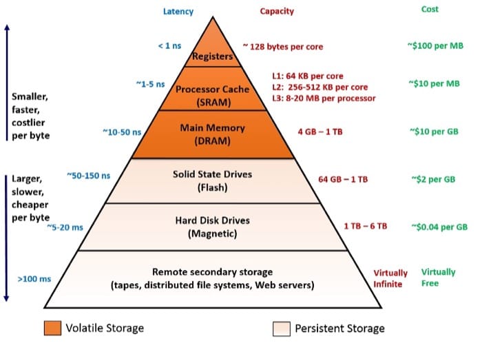
From here, there is a significant leap in terms of capacity and access time when going to main memory (DRAM). Current DRAM technology allows for access latencies of 50-70 nanoseconds, and consists of multiple gigabytes. DRAM costs about ~$10-30 per GB, allowing for a few gigabytes of storage in personal computers, and up to a terabyte in servers. Recall that all of the memories described thus far are all volatile memories. The data stored in these memories exist as long as they are powered ON. When switched OFF, they lose all information.

The next order of magnitude difference is observed in disks, which can take anywhere between 10s of nanoseconds to 100s of milliseconds to fetch a given item, depending on the type of storage device used. Finally, there is the network, which can connect machines that are in the same rack or can go across countries. The access latencies here can vary significantly, depending on the technologies used and the distance. Disks are non-volatile and persist data even when switched off.

Types of Storage Devices

Magnetic Disks

Magnetic disks have been the most cost-effective and popular storage systems for many decades now, but are slowly ceding their dominant position to solid state drives. Magnetic disks consist of one or more spinning magnetic platters and a movable read/write head that floats above the platters. Magnetic disks are extremely dense and cheap. At the time of writing, 6 Terabyte drives are available in the 3.5" desktop form factor for about $270, which translates to about 4 cents per gigabyte. This makes magnetic disks one of the cheapest on-line storage technologies available (as opposed to offline/removable technologies such as tapes and optical discs).

However, Magnetic disks are among the slowest storage technologies. Typical access latencies on modern disks range between 5-20 milliseconds. The main reason for the performance of magnetic disks is the fact that there are moving parts involved during reading and writing of data. As illustrated in Figure 4.4, magnetic disks are organized as a collection of sectors, tracks, and cylinders. In particular, a surface on a typical disk drive is divided into a number of concentric tracks. Each track is divided into a number of equal-sized sectors. The data stored at sectors are read and written using a set of read and write heads, with one head per surface. The set of tracks selected by the disk heads at any one time is called a cylinder. The data at sectors are accessed by moving disk heads to the appropriate cylinder (the time required for this task is called seek time) and then waiting for the disk to rotate until the desired disk sector is under one of the heads (called the rotational time). The time required to access a sector (i.e., seek time + rotational time) depends on the distance of the current position of the disk heads from the desired sector.

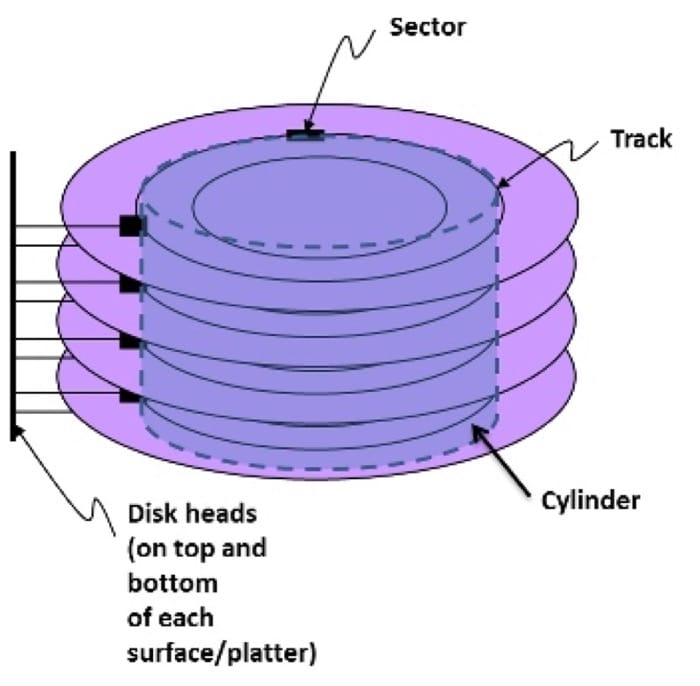
As a result, magnetic storage disks are slow, particularly for random reads and writes, as the head must keep moving to different areas on the disk to read information, increasing the overall access time. However, they are cheap, and they are the main storage technology used in large-scale storage systems. Magnetic storage tends to be the main storage device located at the end of the spectrum, responsible for persisting large amounts of data in a cost effective manner.

Solid State Disks (SSDs)

The emergence of the NAND flash technology has brought increased performance and reduced prices to solid state storage in the past decade or so. Solid state drives, unlike magnetic disks, do not have any moving parts, and are nearly an order of magnitude faster than magnetic disks for random reads and writes. SSDs have access latencies that are an order of magnitude better than magnetic disks (70-150 nanoseconds for sequential operations), but cost significantly more (~$2 -$5 per GB).

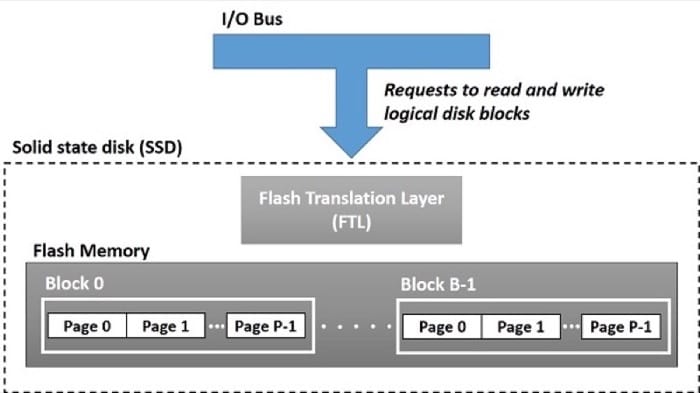
Solid state disks, however, have their own performance and reliability issues. Due to the nature of NAND flash technology, writes to SSDs require an expensive erase cycle that erases an entire page of data (Figure 4.5), which takes time and wears out the flash medium over time. SSDs internally contain logic to level the wear of the medium by spreading out the writes over multiple pages and blocks on the disk. As discussed in Unit 2, there are multiple SSD technologies available in the market, where the primary tradeoff is cost vs. performance and disk life.

As a result, SSDs have different performance characteristics than rotating disks. Sequential reads and writes (where the CPU accesses logical disk blocks in sequential order) have comparable performance, with sequential reading somewhat faster than sequential writing. However, when logical blocks are accessed in random order, writing is an order of magnitude slower than reading, mainly due to the nature of the erase logic in SSDs.

DRAM as a Storage Device

The constant expansion of DRAM sizes, coupled with the drop in price per gigabyte has led to the emergence of in-memory storage systems. In memory storage systems offer an order of magnitude faster performance than traditional disk-based storage systems, but with one big caveat - durability. In memory storage systems typically have fairly complex schemes that stream data down to durable storage in order to persist the data for recovery and fault tolerance purposes. We will explore these types of systems in detail later in this module.

Storage Class Memories / Non-Volatile Memories

A number of technologies are emerging that aim to bridge the performance gap between the volatile DRAM and the non-volatile SSD/Magnetic disks. Dubbed storage class memories, these devices are aiming for access latencies that are within an order of magnitued of DRAM, allowing for the rapid movement of data, while retaining persistence properties of SSDs/magnetic disks, and having much higher storage densities than DRAM. Along with improved versions of NAND Flash memory, technologies such as memristors, phase change memory and others are competing gain a foothold in this space. SCM/NVM class memories are an ongoing developement which we expect to become part of the memory hierarchy soon.

Storage Abstractions

Abstractions in Storage

On a fundamental level, data are stored in binary encoding on some medium (such as the ones described in the previous page magnetic or solid state media). The challenge is to systematically organize the data in systems that are accessible to users and applications. These systems of organization provide abstractions to users and applications in the form of files on a file system, or as entities in a database.

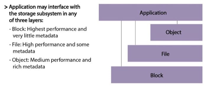
It is important to note that applications can interact with any layer of the abstractions, including the block-level (which is rare for any non-system program). Block devices offer the highest performance but have the least metadata, making it very difficult to write programs using this layer. Many applications interact with a file system, and for applications that require more metadata, database systems may offer a better and more efficient abstraction to manage data.

Block Devices

In the previous pages you learned about different types of data and storage devices. Although there will always be data residing in various cache memories to improve performance, eventually it has to be stored on a persistent (sometimes called nonvolatile) medium such as Magnetic Disks or SSDs. Since these devices typically have a non-trivial architecture and layout, the interface presented to the operating system is a generic block device.

A block is simply a collection of bytes that is grouped together. The block size indicates how many bytes are in that block, such as 512 bytes, 64kiB, or 1MiB. Block sizes are usually represented as a power of 2. A single block is the smallest unit that can be addressed, so all of the bytes in a block must be read or written at the same time. This is similar to how a CPU accesses memory in words (either 32 bits or 64 bits) at a time; if you want to modify a single byte of data either in registers or main memory during a CPU instruction, you have to read 8 bytes (in case of a 64-bit CPU), modify 1, and then write the new word (1 new byte + 7 original bytes) back to memory. This process is amplified with blocks, so an application that modifies a single byte requires reading, say, 512 bytes, modifying 1 byte, and then writing back 512 bytes. This is a rare case, since applications typically read a number of contiguous blocks at a time and may be cached somewhere along the memory hierarchy.

A block device provides an OS access to blocks through an interface. In practice, block devices can be physical or virtual, and can be local or remote. A taxonomy of block devices along with examples are presented below:

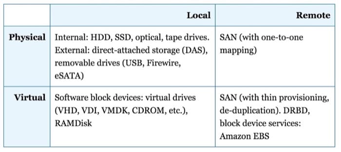
Physical storage devices correspond to a one-to-one mapping of physical storage blocks to the blocks exposed to the OS. Virtual devices abstract the details of a physical block device from the OS and instead present a virtualized block device to the OS.

Local storage refers to block devices that are directly connected to a computer. These can be either internal devices (connected via SCSI or ATA interfaces) or external devices (connected via USB, Firewire, eSATA, etc.). Remote storage is storage that is not directly attached to a computer, but is accessed through a network (using protocols such as Fibre Channel (FC) or iSCSI).

Physical block devices that are local to a computer include the common examples of hard disk drives, optical drives, and tape drives that are directly connected either through an internal interface or an external interface. The best example of a physical block device that is connected externally to a computer is a SAN with one-to-one mapping between the blocks allocated on the SAN to the blocks accessed by the OS.

Virtual block devices that are local to a computer include any block device that is represented as a file. Examples include virtual machine disk images such as Virtual Machine Disk (VMDK, VMware’s virtual disk format), Virtual Disk Image (VDI, VirtualBox’s disk format), and Virtual Hard Disk (VHD).

Remotely accessed virtual block devices include SANs, which export block devices that do not have a one-to-one correspondence with physically allocated blocks. For example, SANs can thinly provision a block device of 1TB to a server, but the actual disk space used on the SAN is the exact amount of storage used by the server at the moment. When an OS writes additional data to the block device, the block allocations within the SAN increase. SANs also have features such as de-duplication, which identifies identical blocks and stores only a single copy.

File Systems

One basic abstraction of storage is the concept of files and file systems. A file, in the context of storage, can be thought of as a block of information that is made available to computer programs. A file system is an abstraction to users and applications that includes the associated data structures to store, retrieve, and update a set of files. A file system typically manages access to its data and metadata (metadata is additional information and parameters that describe the files). File systems have a myriad of responsibilities, ranging from space management, naming, metadata management, and access control to maintaining the reliability and integrity of the files stored in the system.

File systems can be categorized into many types. Figure 4.7 illustrates the hierarchical taxonomy of file systems as defined by the Storage Networking Industry Association (SNIA).

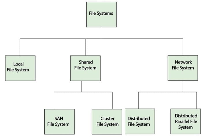
Based on their architecture and implementation, file systems can be broadly defined as

• Local file systems: These are file systems that are designed to be operated on a one or more disks, granting access to a single instance of an operating system to storage devices. Examples include FAT, ext, HFS, ReiserFS etc.
• Shared file systems: These are special purpose file systems that allow multiple disks to be pooled into a group of available block devices to be shared among multiple machines over a network. Examples include IBM's GPFS and SanFS.
• Network file systems: Network file systems are higher-level storage services offered to applications (as opposed to plain block devices in Local and Shared file systems). Examples include CIFS, NFS, among others. We will explore, in detail, a special class of network file systems called Distributed File Systems in this module.

Databases

Another layer of abstraction in storage systems is Databases. Databases are typically run on top of file systems, but there are instances where databases are run directly on top of block devices in order to improve performance, but these are rare. As we will see in detail in this module, databases are designed to store and retrieve information for applications. Databases have higher visibility into the data, sometimes allowing for complicated queries and operations on the data.

References

1. Thomas Rivera (2012). "The Evolution of File Systems." SNIA Tutorial.

Local File Systems

In a local file system, the file system is collocated with the server that runs the application. Owing to the nature of the file system, local file systems have limited scalability and do not allow for data sharing across different clients over a network on their own (Figure 4.8).

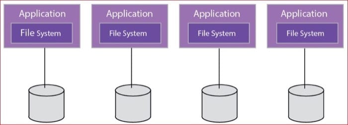
Data stored on a disk are typically represented as blocks, or a contiguous, unstructured collection of bytes. Local file systems provide an abstraction of files, which are simply a collection of blocks that represent a file.

Applications using local file systems are not concerned with how files are physically represented on storage media, the amount of data transferred to or from the application per file request (called record size), the unit by which data is transferred to or from storage mediums (called block size), and so on. All such low-level details are managed by local file systems and are effectively abstracted from user applications. In principle, local file systems are the basic building substrate of every file system type on the cloud. For instance, distributed file systems (e.g., Hadoop Distributed File System which mimics the Google File System) [2] and parallel file systems (e.g., PVFS) are built and executed on multiple cooperative local file systems. Moreover, how well a virtual machine or a physical machine can survive software and hardware crashes on the cloud and on other systems depends partly on how well the local file systems are designed to handle such crashes. In short, practically every file system, whether shared or networked, relies on local file systems.

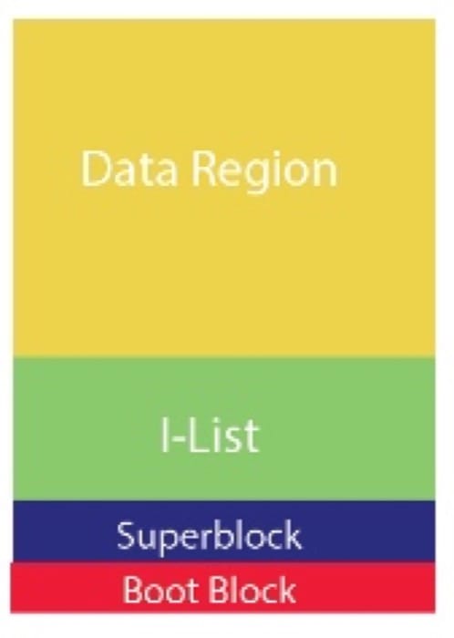
The UNIX file system is a classic local file system that was designed in the 1970s and has since been in widespread use in many forms (FFS, EXT-2, etc.). Although the data within a file is distributed as a series of blocks on a storage device, the file system maintains the abstraction of the file along with its associated data. As shown in Figure 4.9, a basic local file system includes a boot block, a superblock, an I-list and a data region. The boot block holds the boot program that reads the operating system’s (OS’s) binary image into the memory when the OS is booted. In essence, the boot block has nothing to do with any of the file system management processes and functionalities. The superblock describes the layout and the characteristics of the local file system, including its size, the block size, the blocks’ count, the I-list size and location, and so on.

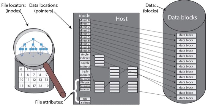
In the I-list, the state of each file is encapsulated as a UNIX inode (index node; Figure 4.10). The inode acts as the primary data structure of a file and stores the metadata about a file, including pointers to the individual file blocks in storage, ownership and access control lists, timestamp of the last access of the file, and so on.

Examples of local file systems include NTFS, FAT, and EXT. The scalability, performance, and sharing limitations of local file systems can be overcome by using shared/networked file systems.

POSIX I/O Standards

The Portable Operating System Interface (POSIX) is a family of standards that defines operating system (OS) interfaces for many UNIX and UNIX-like OSs. The POSIX file system standards are often used to describe the capabilities expected from a file system that can be used in UNIX and UNIX-like OSs.

POSIX defines the following standard operations on files: open, read, write, and close. In addition, the POSIX standards allow such file systems to be directly mounted in a UNIX or UNIX-like OS without having a special-purpose driver/client process to manage the file system.

Kernel-Level vs. User-Level File Systems

Kernel level file systems are file systems which contain a kernel level API, which also means that the code that interacts with the file system resides in the Kernel. In UNIX and UNIX-like operating systems, these APIs are loaded in as modules. Kernel-level file systems in UNIX-like operating systems are typically POSIX compliant and are usually limited to local file systems.

User-level file systems operate in user space as opposed to the kernel space. Such file system interfaces allow for a file system API to be portable and allow for installation in a much broader set of clients. Many distributed and networked file systems are designed to work in user-level, with one exception being AFS, which uses a kernel-level driver in Linux.

Design Considerations in Local File Systems

To understand how local file systems are designed, it is important to understand the underlying storage medium. In this discussion, we assume a spinning disk as storage medium.

Local file systems are designed to minimize seek and rotational times upon allocating disk capacity for files to improve system performance. Local file systems can also maximize the amount of useful data transferred after incurring the seek and rotational times. Performance is a main criterion for designing an effective local file system. Storage mediums such as disks and magnetic tapes do not provide uniform access times as primary storages (e.g., memory or caches). Consequently, a local file system should leverage the underlying storage medium to its fullest in order to achieve acceptable system performance and avoid undue waste of space. Avoiding undue waste of space is crucial, especially on the cloud where system resource utilization is of great significance.

Performance

To improve performance, local file systems can employ various strategies. First, local file systems can keep a number of block addresses in a file’s inode (specifically, in its diskmap). Local file systems can cache inodes in memory to reduce the number of disk accesses needed to read/write block locations. Second, to maximize the amount of useful data transferred, local file systems can make block sizes larger. Third, to minimize seek time, locality can be exploited. Specifically, blocks that are likely to be accessed in the near future can be kept in close proximity to one another on the disk, which means the blocks of each file must be stored as close together as possible. Furthermore, because inodes are accessed in conjunction with their data blocks, they must be stored close to each other. And because the inodes of a directory are often examined all at once (e.g., ls –la), the inodes of files at a single directory should be kept close to each other. Fourth, to reduce rotational latency, the blocks of a file in a cylinder (if any) should be arranged in a way that, after the seek time, they can all be read without further rotational delays. This arrangement enhances performance, especially if blocks are requested sequentially. If, however, the blocks are requested randomly, it becomes difficult to leverage such a block arrangement at a cylinder to minimize rotational latency. Finally, when a local file system is fetching a requested block, it can simultaneously prefetch blocks that are likely to be accessed in the near future. In fact, many local file systems (e.g., Ext2 and later versions) use a multiple-block-at-a-time strategy known as block clustering whereby eight contiguous blocks at a time are allocated. Blocks can also be buffered or cached for future references by the OS.

Although file systems were traditionally built to optimize performance on magnetic hard disks, many current file systems have operating modes for SSDs, which does away with some of the optimizations targeted at disks, and introduces new features for improved performance and wear management on SSDs.

Dependability

Another major criterion for designing effective local file systems is dependability. Dependability is also of a main concern for cloud storage. Local file systems should be dependable; that is, stored data must be accessible whenever it is needed. Hence, data should effectively tolerate software and hardware crashes. In addition, local file systems must ensure that the stored data are always consistent. Writing, creating, deleting, and renaming a file might require a number of disk operations that affect both data and metadata. To make sure that the underlying local file system is crash-tolerant means to ensure that any of these operations shall take the system from one consistent state to another. For instance, moving a file from one directory to another, which involves create and delete operations, might result in an inconsistent file system state. In particular, a crash might occur while the file is being moved, leading to the disappearance of the file in the two directories, the original and the projected one. To avoid this risk, the local file system can first create the file at the projected directory and subsequently remove it from the old one (after the file is committed at the new directory).

Multi step File System Operations

Some file operations might require multiple read or write steps, known as multi step file system operations. For instance, writing a large amount of data to a file might result in a number of separate disk operations (which is common on clouds). If a crash occurs before all of the required data is written, the local file system will end up in a state with only part of the write operation completed. A popular approach to deal with multi step operations is to use atomic transactions. With atomic transactions, if the system crashes during any step of a given multi step operation, the effect (probably after some recovery operations) is as if the whole operation either took place completely or did not occur at all. Transactions are a standard fare in database systems and are discussed in detail in the database section.

One basic scheme to implement atomic transactions in local file systems is called journaling. In journaling, the steps of a transaction are first written onto disk in a special journal file. Once the steps are safely recorded and the operation is committed (i.e., totally completed), they can be applied to the actual file system. If a crash occurs while the steps are being applied to the file system, the steps can be easily recovered from the journal file (assuming it is constantly protected from failures). This technique is known as the redo or new-value journaling. Even if the system crashes while the steps are being applied to the journal file, the already recorded steps in the journal file can be discarded and the actual file system will remain intact. The journaling approach guarantees that the whole operation will take place either completely or not at all.

Expanding a Single File System over Multiple Disks

To enhance dependability and/or performance, a local file system can be used with multiple disk drives. Video 4.3 covers the various techniques used to expand a file systems over mulitple disks

Video 4.3: File System Expansion

The three main reasons for expanding disk drives are

1. To attain more disk storage
2. To store data redundantly
3. To spread blocks across multiple drives so they can be accessed in parallel, thereby improving performance

Multiple disks can be transparently exposed to the local file system as a single disk using what is known as a logical volume manager (LVM). If we assume two disks, an LVM can present a large address space to the local file system and internally map half of the addresses to one disk and the other half to the second disk. To provide redundancy, an LVM can store identical copies of each block on each of the two disks. Doing so necessitates passing read and write operations through the LVM. For each write, the LVM updates the two desired identical copies on the two disks. For each read, the LVM forwards the request to the disk that is less busy. Finally, parallel accesses with multiple disks can be carried out using a technique called file striping. With file striping, a file is split into multiple units, which are subsequently spread across disks to enable parallel accesses to the file.

Data can be striped in different ways depending on the stripe unit (the level at which data is striped across multiple disks). In block-level striping, the stripe unit is a block of data. The size of a data block, which is known as the stripe width, varies with the implementation but is always at least as large as a disk's sector size. When it comes time to read back this sequential data, all disks can be read in parallel. In a multitasking operating system, there is a high probability that even non-sequential disk accesses will keep all of the disks working in parallel. In byte-level striping, the stripe unit is exactly one byte. With bit-level striping, the stripe unit is exactly one bit.

RAID

As discussed in the data center module, multiple disks can be combined into a single logical drive using a RAID organization. RAID 0 stripes data at the block level over multiple disks with no redundancy. RAID 1 mirrors data of one disk to another and typically halves the capacity of an array. RAID 2 provides bit-level striping with hamming codes stored on parity drives. RAID 3 provides byte-level striping with parity information stored on dedicated parity drives. RAID 4 provides block-level striping with dedicated parity drives. RAID 5 provides the same block-level striping as RAID 4 and 1, but the parity information is distributed among all drives in the set. Finally RAID 6, is the same as RAID 5 but with parity blocks written twice so RAID 6 can tolerate up to two disk failures within a set. Combination RAID configurations, such as RAID 1+0 and RAID 0+1, are also possible for a mixture of performance and reliability guarantees.

Storage Area Networks (SANs)

In an enterprise IT environment, it is typical for storage to be consolidated so that it can be pooled and shared across multiple servers. Storage devices can be shared among multiple servers using a storage area network (SAN). A SAN is a dedicated network that provides access to consolidated, block-level data storage (Figure 4.11). The consolidated, block-level storage is typically in the form of a disk array. The disk array can be configured with some form of RAID, depending on the performance and reliability required. Servers typically access the SAN using a protocol such as iSCSI or Fibre Channel (FC). The servers that use a SAN see a logical block device, which can be formatted with a file system and mounted in the server. The application server can then use the externally stored logical blocks in the same way it would use locally stored blocks. Thus, the logical placement of the data is different from its physical placement.

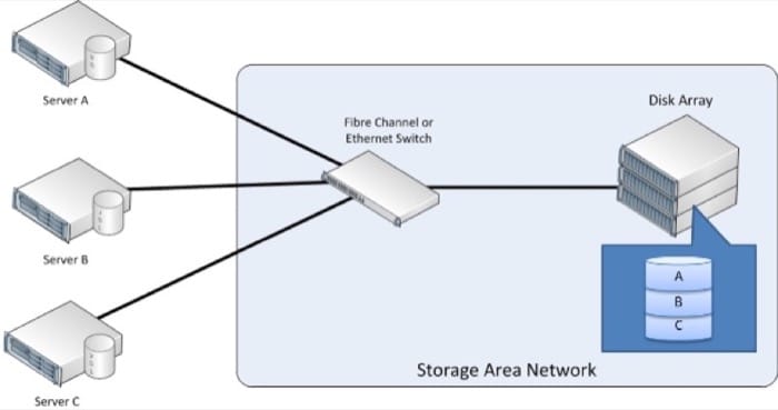
Although the servers share the disk array, they cannot physically share data residing on the disks. Instead, portions of the SAN (identified as logical unit numbers, or LUNs) are carved out and provided for the exclusive use of each server.

References

1. Thomas Rivera (2012). "The Evolution of File Systems." SNIA Tutorial.
2. Sanjay Ghemawat, Howard Gobioff, and Shun-Tak Leung (2003). "The Google File Systems." 19th ACM Symposium on Operating Systems Principles.

Distributed File Systems

Switching gears now, we will discuss distributed file systems. A distributed file system is a file system that has files distributed among multiple file servers (Video 4.4).

Video 4.4: Distributed File Systems

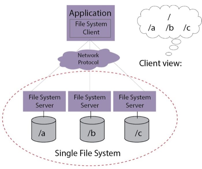
It is important to note that in a distributed file system, the client views a single, global namespace that encompasses all the files across all the file system servers (Figure 4.12).

As with a shared file system, DFSs require metadata management so that clients can locate the required files and file blocks across the file servers. The metadata server can be asymmetric (single metadata server) or symmetric (metadata servers on each file server), similar to shared file systems.

Origins and Evolution of Distributed File Systems

Examples of DFSs include the Andrew File System (AFS). AFS is a distributed file system that enables cooperating hosts (clients and servers) to efficiently share file system resources across both local area and wide area networks. AFS consists of cells, an administrative grouping of servers that present a single cohesive file system. Cells can be combined to form a single global namespace. Any client that accesses data from AFS will first copy the file locally to the client. Changes to the file will be made locally as long as the file is open. When the file is closed, the AFS client will sync the changes back to the server. An evolution of AFS is CODA, which is a distributed file system that improves on AFS, particularly with respect to sharing semantics and replication.

In 2003, Google revealed the design of its distributed file system, called GFS [2] , which was designed from scratch to provide efficient, reliable access to data using large clusters of commodity hardware. GFS is designed to store very large files as chunks (typically of size 64MB), in a replicated fashion. Although GFS has a singular client view like AFS, the location of file chunks is exposed to the user, given opportunities to fetch files from the closest available replica. GFS is the inspiration behind the Hadoop Distributed File Systems (HDFS), which is covered in detail in the next module.

Design Characteristics in Distributed File Systems

DFSs are typically deployed on multiple file-sharing nodes and are intended for use by multiple users at the same time. As with any shared resource, multiple design considerations must be considered:

• Fault tolerance
• Replication
• Consistency
• File-sharing semantics

Shared and networked file systems must be designed with failures in mind. Fault tolerance can be defined as the ability of a system to respond gracefully to unexpected hardware and software failures. In the case of file systems, fault tolerance requires the file system to respond gracefully to disk, node, and network failures. With shared and networked file systems, the odds of a disk failing increase with the number of disks in the array/pool. At the hardware level, faults can be tolerated by using some form of RAID.

At the file system level, data in distributed systems may be replicated; the same data may be maintained on one or more nodes in the distributed file system. This replication is done in order to

• Improve performance (a client can potentially find a replica that is nearest to its location).
• Enhance the scalability of the system (simultaneous requests for data can be handled by different servers).
• Enhance reliability (replicas can provide fault tolerance and provide a checksum mechanism to ensure the integrity of the data).

Replication is the primary mechanism to deliver fault tolerance in DFSs. The capacity of a DFS is usually impacted by the replication factor (the number of active replicas to be maintained). For example, a DFS configured with a raw capacity of 15TB can store only 5TB of data if all the data is triple replicated.

Replication poses the additional challenge of consistency. In a large distributed system, updates to files must be applied to all replicas. The level of consistency supported in a DFS also affects client interactions with the file system.

When a resource, such as a file, is shared between multiple users, it is necessary to define the semantics of reading and writing to the file. Following are some of the semantics that can be implemented with a DFS:

• UNIX semantics: In UNIX semantics, a read operation performed immediately after a write operation will always return the value that was just written. UNIX employs the strictest file-sharing semantics in file systems. With UNIX semantics, performance may be affected because reads and writes may have to be serialized to ensure that all file system operations are consistent.
• Session semantics: In session semantics, changes to an open file are initially visible only to the process that modified the file. Once the file is closed, the changes are made visible to other processes. Session semantics relaxes the strict requirements employed by UNIX semantics, but the question of conflict handling emerges: When two clients are simultaneously editing the same file, whose session is honored? Some approaches honor only the last client to close the file, while others might even be unspecified.
• Immutable semantics: In immutable semantics, files can be written only once to a file system and cannot be reopened for further modification. Files can be deleted, or a new file can be created to replace the old one. If two or more processes try to replace the file simultaneously, the file system should resolve the tie through first in, first out (FIFO) order or in a non-deterministic fashion. The file system must also account for the possibility that one of the processes can replace a file while another is busy reading it. In this scenario, the file system should either arrange for the reader to continue using the old file or detect that the file is now replaced and not allow the reading process to continue accessing the file.
• Atomic transactions: In an atomic transaction model, the start and end of sequences of read and write operations are marked as being a transaction in which the changes to files happen atomically (changes are either committed as a whole or not committed at all).

References

1. Thomas Rivera (2012). "The Evolution of File Systems." SNIA Tutorial.
2. Sanjay Ghemawat, Howard Gobioff, and Shun-Tak Leung (2003). "The Google File System." 19th ACM Symposium on Operating Systems Principles.

Databases

File systems are typically used to store arbitrary data as files on disks with some form of metadata (such as a filename) used to identify and locate these files. File systems offer rudimentary search and indexing capabilities, and searching the contents of files to find the information you need is often an involved and laborious process. When the data is amenable to structuring, it is typical to organize it in a database, using a well-defined model (also known as a schema). Video 4.5 provides an overview of Databases:

Video 4.5: Databases

A database consists of an organized collection of data for one or more uses, typically in digital form. Databases are one of the most popular information storage and retrieval methods for many types of applications, including financial, manufacturing, business, and personnel data.

Databases have evolved over the years, starting with the navigational model in the 1960s, which stored data as records with pointers that linked to the next and/or previous record in the database. Examples include the Codasyl approach, which eventually evolved into the Common Business Oriented Language (COBOL). The Codasyl approach was based on the "manual" navigation of a linked data set, which was formed into a large "network" of linked data, much like a circular linked list. When the database was first opened by a program, the program was handed back a link to the first record in the database, which also contained pointers to other pieces of data. To find any particular record, the programmer had to step through these pointers one at a time until the required record was returned. Simple queries that aggregate information across records required a complete scan of the entire database—concepts such as search and indexing did not exist then. The Codasyl approach was appropriate in an era when magnetic tapes were the primary mode of nonvolatile storage, which could be read only sequentially and had no random access properties.

The emergence of the relational database model and the subsequent development of IBM's Systems R was a major milestone in database system development. For many decades Relational database systems were the only databases in wide use, and are extremely successful. With the growth of the Internet and the need for massively scalable systems that can service millions of simultaneous requests, NoSQL database systems emerged, starting with the likes of Google's BigTable and Amazon's dynamo. However, of late, a class of relational database systems have emerged, re-architected from scratch to try to combine the strengths of the two models.

Types of Database Systems

Current database systems can be classified into the following types:

Relational databases are the classical database systems which have been around for decades. They follow the relational model of representing data as relations between entities. Relational database systems typically have a rigid schema, use the Structured Query Language (SQL) as the interface to interact with the database, and typically have strong ACID properties.

NoSQL databases are a new breed of databases which are markedly different from relational database systems. NoSQL systems typically do not enforce a strong schema or relational model of the data, and instead provide a different abstraction (like a key-value store), instead of a SQL-like interface. NoSQL databases are focused on scalability and performance, and typically do not have strong transactional guarantees for database operations.

NewSQL is a class of modern relational database systems that seek to provide the same level of performance and scalability as NoSQL systems but while maintaining some degree of ACID properties that relational database systems offer.

Designing Databases - Schema and Scalability

Databases, as you can imagine, encompass a broad range of applications and requirements. To this end, we will discuss a few specific design patterns that database creators have to make when creating their database systems.

Schema Enforcement

Database systems, in general, require some information regarding the types and structures of the data to be stored in the database. With relational database systems, the schema is formally defined in terms of :

1. Tuples (Rows), which consist of Attributes (Columns) all of which are defined to be a certain type.
2. A Relation (table), which consists of multiple tuples of the same type.
3. Constraints, which define a set of rules on tuples, attributes and relations.

Schema are not mere guidelines, but are enforced in relational systems. Schema-based databases have the following advantages:

1. Schema express the data model in a manner which allows for complex operations and queries to be constructed. For example, a join (where data is inferred from two or more distinct tables, is relatively easy to express in a relational database).
2. Schemas can contain constraints which can be used to enforce program logic at the database level. For example, simple constraints can check if a person's age is a positive number, while a bank ledger implemented as a set of tables in a relational database can enforce the property (using a complex constraint), that the sum of all credits and debits in the system must equal to zero. The system can automatically reject or return transactions that violates these constraints.
3. Relational systems take advantage of the information provided in the schema to construct elaborate and efficient query plans, allowing the database to efficiently answer queries regarding the data stored.

However, the rigid enforcement of a schema is also a barrier to flexibility. As an application evolves, changing the schema of a table that is already populated with rows is difficult, if not impossible, depending on the table and the constraints provided.

On the other hand, there are systems that have either flexible schema, or no schema whatsoever. An example of a system with practically no schema is a generic key-value store, which basically acts as mapping between keys or a certain type and an associated value. Some key-value stores are very flexible; they allow for any arbitrary binary data to be stored under a particular key. Some key value stores, such as Dynamo, require that the type of the key (i.e. string, integer, etc.) should be made explicit when creating a new table. Some systems allow for nested values to be present in data attributes, typically stored as JSON or XML.

Another variation is systems like BigTable and HBase, which have a semi-flexible schema. These systems require the number of columns to be declared when a table is created, but a column can have any number of nested sub-columns. These systems will be covered in detail in the next module.

Transaction vs. Analytical Processing

A key design choice that needs to be made when optimizing a database system is to optimize for the common case of the type of queries that it will receive. There are two main patterns in database workloads that have emerged.

Transactional workloads, also known as Online Transactional Processing (OLTP), are workloads that are mainly composed of short on-line transactions. OLTP workloads mainly consist of insertions, updates and/or deletions. The emphasis on OLTP systems is on fast query processing and maintaining data integrity in environments where there is simultaneous access. A good example of an OLTP workload is financial transactions. Queries will typically involve only a few tables and rows and will not require vast scans of the database.

On the other hand, certain systems aggregate and analyze data in order to gain insights and derive information from the data. Such systems are called Online Analytic Processing (OLAP) systems. OLAP systems generally involve a lower volume of transactions but individual queries may be complex and involve aggregate computations that span multiple rows and multiple tables. Typical OLAP queries thus are significantly longer running than OLTP queries.

Video 4.6 provides an overview of OLTP vs. OLAP:

Video 4.6: OLTP vs. OLAP

Scalability

Over time, when a database system's user base and data grows, it may require some form of scaling, which would expand the capacity and/or the performance of the database system in order to support more users or data, or both. Database scaling is complex for a variety of reasons which we will cover in detail in Video 4.7:

Video 4.7: Database Scaling

Vertical Scaling

Vertical scaling (or scaling up) is the process of increasing a database’s capacity or ability to handle load without adding more hosts. This can be done by hardware upgrades such as a faster CPU, increased RAM, or disks with more capacity and/or more I/O operations per second (IOPS). The scalability with vertical scaling is limited by the amount of CPU, RAM, and disk that can be configured on a single machine.

Horizontal Scaling

Horizontal scaling (or scaling out) means the scaling of databases by adding more nodes to handle database queries. Different RDBMS products offer different ways of scaling out, including replication and database sharding. With replication, the same data is stored across multiple nodes. This enables the RDBMS to handle additional requests in parallel, thereby increasing the number of transactions per second. This approach works when the database is read-heavy. In sharding, a large table is partitioned across multiple nodes (typically on an index or key). The amount of data shared across nodes is limited in this case, and limited sharing is preferred because it reduce issues with consistency of replicated data.

Replication is the process of duplicating data over multiple servers in order to increase the number of available paths to individual pieces of data. Data can be replicated for performance, availability and/or fault tolerance reasons. Replicated data allows for faster performance, particularly for reads, as replication allows for parallel access to multiple copies of the same data. Replication assists in availability and fault tolerance as data is available in a backup location should a part of the database system fail.

Another method, that is orthogonal to replication, it sharding. Sharding is the process by which data is partitioned into sections (known as shards) and distributed over multiple database systems. In contrast to replication, each shard acts as the single source for the subset of data contained by it. Sharding is a technique that is specifically used to improve the performance of databases, and in particular, write performance.

In an ideal case, a sharded database will evenly spread out the data across all partitions, but this is difficult to achieve as the data distribution across all partitions should be more or less balanced. A popular technique that is the mainstay of many current database systems is consistent hashing.

Consistent hashing is a special kind of hashing technique which allows for a hash table to be expanded in an efficient manner. If K is the total number of keys and n is the number of buckets in a given hash table, consistent hashing requires only K/n keys to be remapped on average every time a new bucket is added to the hash table. More details on consistent hashing can be read here [1] .

Some systems use a combination of replication and sharding to provide high performance while maintaining high availability and fault tolerance. However, when using replication, a major concern is consistency, which will be discussed next.

References

1. Karger, David and Lehman, Eric and Leighton, Tom and Panigrahy, Rina and Levine, Matthew and Lewin, Danielr (1997). "Consistent Hashing and Random Trees: Distributed Caching Protocols for Relieving Hot Spots on the World Wide Web." Proceedings of the Twenty-ninth Annual ACM Symposium on Theory of Computing.
2. Eric Brewer (2000). "Towards Robust Distributed Systems." Proceedings of the Annual ACM Symposium on Principles of Distributed Computing.

Designing Databases - Consistency and the CAP Theorem

Consistency

Without replication, consistency is not a concern. Replication entails maintaining multiple copies (or replicas) of the same data across multiple machines, whereas consistency provides a system-wide consistent view/state of replicas across multiple clients/processes. As pointed out earlier, data items are replicated for two primary reasons: performance and reliability. Regarding performance, replication is crucial when the system needs to scale in numbers (as is mainly the case with storages in private and public clouds) and in geographical areas (as is usually the case with storages in public clouds). For instance, when an increased number of processes must access data that are managed by a single storage server, performance can be improved by replicating the data across multiple servers (instead of having only one server) and subsequently dividing the work across the servers. This division allows requests to be served concurrently and thereby increases system speed. In contrast, replication across geographical areas (e.g., as applied by Amazon S3) can be ensured by replicating copies of data in the proximity of the requesting processes to minimize data access times. Concerning reliability, replication makes it possible to provide better fault tolerance against corrupted and lost data, a key requirement on the cloud. In particular, if a replica is lost or corrupted, another valid replica (if maintained) can be alternatively accessed.

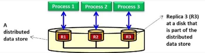
Replication produces multiple replicas of data, and consistency ensures that those replicas remain uniform so that different processes can access (i.e., read and write) them. Specifically, a collection of replicas are considered to be consistent when they appear identical to concurrently accessing processes. The ability to handle concurrent operations on replicas while maintaining consistency is fundamental to distributed storage in general and cloud storage in particular. In this unit, consistency is discussed in the context of read and write operations performed on shared replicas in a distributed data store (Figure 4.13). The distributed data store can be a DFS, a parallel file system, or a distributed database. Consistency can be achieved by employing a consistency model. We define a consistency model as a contract between processes and the distributed data store, which implies that if processes agree to obey certain rules, the distributed data store promises to enforce those rules. Video 4.8 covers a number of consistency models.

Video 4.8: Consistency Models

We discuss three consistency models in detail in this unit: sequential consistency, causal consistency, and eventual consistency.

Sequential Consistency

Also called strong or strict consistency, sequential consistency entails propagating updates to all replicas immediately, which typically requires applying updates on related replicas in a single atomic operation, or transaction. In practice, implementing atomicity across widely dispersed replicas in a large-scale distributed data store is inherently difficult, especially if updates are to be completed quickly. The difficulty stems from the unpredictable access latencies imposed by the underlying storage network and the lack of a global clock that can be utilized to order operations rapidly and accurately. To address this problem, the requirement of executing updates as atomic operations can be relaxed. Relaxing consistency requirements means that replicas need not always be the same in all locations. Whether or not consistency relaxation is acceptable depends on the application that is running over the distributed data store. Specifically, relaxing consistency requirements depends on the read and write access patterns of the application and the purpose for which replicas are used. For instance, browsers and Web proxies are often configured to store Web pages in local caches (this is a type of replication because multiple copies are maintained for the same Web page) to reduce access times for future references. It is acceptable in some situations that users receive outdated Web pages as long as, eventually and rapidly enough, the Web pages will be upgraded to the most up-to-date versions available at the actual Web server(s). Eventual consistency is an example of a model that suits such scenarios.

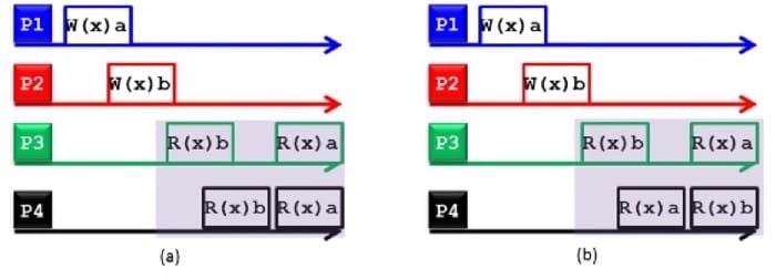
A distributed data store is considered sequentially consistent if all processes see the same interleaving of read and write operations when accessing replicas concurrently. Figure 4.14 demonstrates two distributed data stores: a sequentially consistent data store (Figure 4.14(a)) and a nonsequentially consistent data store (Figure 4.14(b)). The symbols W(x)a and R(x)b denote a write value of a to replica x and a read value of b from replica x, respectively. The figure shows four processes operating on replicas corresponding to data item x. In Figure 4.14(a), process P1 writes a to x, and later (in absolute time), process P2 writes b to x. Subsequently, processes P3 and P4 first receive value b and later value a upon reading x. As such, the write operation carried by process P2 appears to have taken place before that of P1 and of both processes P3 and P4. Nonetheless, Figure 4.14(a) still represents a sequentially consistent distributed data store because processes P3 and P4 experience the same interleaving of operations (i.e., reading first b and then a). In contrast, processes P3 and P4 in Figure 4.14(b) see different interleaving of operations, thus violating the condition of sequential consistency.

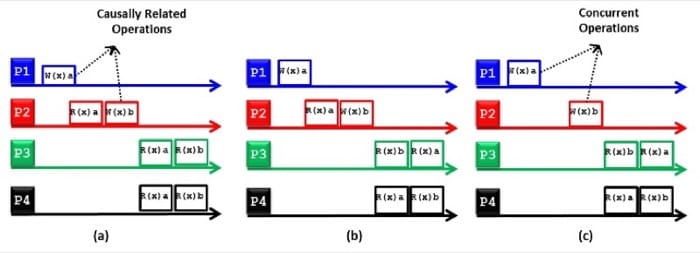
Causal Consistency The causal consistency model is a weaker variant of the sequential consistency model. First, causality implies that if operation b is caused or influenced by an earlier operation a, then every process accessing the distributed data store should see first a and then b. A causally consistent distributed data store enforces consistency across only the operations that are potentially causally related. The operations that are not potentially causally related can appear at processes in any interleaving and are denoted as concurrent operations. Figure 4.15 shows two causally consistent distributed data stores (Figures 4.15(a) and 4.15(c)) and one noncausally consistent distributed data store (Figure 4.15(b)). In Figure 4.15(a), W(x)b performed by process P2 is potentially dependent on W(x)a carried by process P1 because b may be a result of computation involving a read by process P2 (i.e., R(x)a) before writing b (i.e., W(x)b). Thus, the results of the write operations W(x)a and W(x)b performed by P1 and P2, respectively, should appear in the same order at each reading process. Because processes P3 and P4 read first a and then b, they are said to adhere to the causality condition, thus making the underlying distributed data store causally consistent. In contrast, process P3 in Figure 4.15(b) does not abide by the causality condition (i.e., it reads first b and then a), thus rendering the underlying distributed data store noncausally consistent. Last, Figure 4.15(c) illustrates a causality consistent distributed data store because W(x)a and W(x)b are concurrent operations; hence, their results (i.e., R(x)a and R(x)b) can appear in any order in the reading processes, which is the case for processes P3 and P4.

Eventual Consistency The eventual consistency model is considered a weaker form of sequential and causal consistency models. Eventual consistency implies that a write on a replica need not be propagated to all other replicas immediately and can be delayed (or sometimes never propagated) if acceptable by applications. Specifically, if a process P accesses a certain replica, R, N times per a minute, and R is updated M times per minute, then if an application exhibits a low read-to-write ratio (i.e., N << M), many updates to the replica will never be accessed by P, rendering all those updates and the required network communication pointless. In this case, it might be better to apply a weak consistency model whereby R is updated only when accessed by P. That is, it is more efficient to propagate an update in a lazy fashion, whereby a reading process will see an update only after some time has passed since the update took place (not immediately, as is the case with strict consistency). If conflicts resulting from two operations that attempt to write on the same data (i.e., write-write conflicts) seldom or never occur, it is often acceptable to delay the propagation of an update. Conflicts seldom occur with database systems, which typically employ eventual consistency. We discuss database systems in detail in the next section. Note that we presented only part of the story about consistency models. Another part covers how such models are implemented. In this unit, we are concerned only with what these models are and their applicability to cloud storage systems. Nonetheless, we briefly point out that sequential consistency is hard to implement in practice and that it scales poorly. Typically, sequential consistency requires using synchronization mechanisms such as transactions and locks. In contrast, implementing causal consistency involves building a dependency graph that captures causally related operations and enforces those operations across accessing processes. One way to implement such a model is to use vector timestamps. Eventual consistency can be implemented by grouping read and write operations into sessions and using vector timestamps.

ACID Properties in Databases

Databases can offer transactional properties. A transaction comprises a unit of work performed within a database management system (or similar system) against a database. Transactions are treated in a coherent and reliable way independent of other transactions. Transactions in a database environment have two main purposes:

• To provide reliable units of work that allow correct recovery from failures and keep a database consistent even in cases of system failures when execution stops (completely or partially) and many operations on a database remain uncompleted, with unclear status.
• To provide isolation between programs accessing a database concurrently. If this isolation is not provided, the program's outcomes are possibly erroneous.

To better understand the need for transactions in a database, consider the following financial transaction performed on two bank accounts A and B. Suppose a user would like to transfer $100 from account A to account B. This transfer can be represented in two steps:

1. Deduct $100 from account A.
2. Credit $100 to account B.

Suppose a database failure occurs between operations 1 and 2: $100 would have been deducted from account A, but the credit to account B would have not taken place. The accounts, and the database itself, would be in an inconsistent state.

To solve this problem, the operations can be defined as a transaction, as follows:

1. Begin transaction.
2. Deduct $100 from account A.
3. Credit $100 to account B.
4. End transaction.

It now becomes the database’s responsibility to ensure atomicity of this transaction—that the transaction is either successful in its entirety (committed) or not performed at all (rollback). The database should be consistent after the transaction is complete; that is, the database should be in a valid state after the transaction is committed, and any rules defined for records in the database should not be violated (e.g., a savings account may not have a negative balance). Any transactions that are happening concurrently to the accounts must not interfere with each other, thus providing isolation. Finally, the transaction must be durable, which means that the actions performed in the transaction should persist after the transaction is committed to the database. The properties of atomicity, consistency, isolation, and durability are collectively known as the ACID properties of transactions and are expected to be followed by most RDBMS that are used for transaction processing. Video 4.9 provides an overview of ACID properties in databases:

Video 4.9: ACID Properties

• Atomic: The transaction is indivisible—either all the statements in the transaction are applied to the database, or none are.
• Consistent: The database remains in a consistent state before and after transaction execution.
• Isolated: Although multiple transactions can be executed by one or more users simultaneously, one transaction should not see the effects of other concurrent transactions.
• Durable: Once a transaction is saved to the database (an action referred to in database programming parlance as a commit), its changes are expected to persist.

Why you can't have it all: The CAP Theorem

In 1999, Brewer [1] proposed a theorem describing the limitations of distributed data storage called the CAP theorem. The CAP theorem states that any distributed storage system with shared data can have at most two of three desirable properties:

• Consistency: Consistency is a state in which every node always sees the same data at any given instant (strict consistency).
• Availability: A guarantee that every request receives a response about whether it was successful or failed is an availability guarantee.
• Partition tolerance: A network partition is a condition where the nodes of a distributed system cannot contact each other. Partition tolerance means that the system continues to operate normally despite arbitrary message loss or failure of part of the system.

Video 4.9 provides an overview of the CAP theorem:

Video 4.9: The CAP Theorem

The easiest way to understand CAP is to think of two nodes of a distributed storage system on opposite sides of a network partition (Figure 4.16). Allowing at least one node to update state will cause the nodes to become inconsistent, thus forfeiting C. Likewise, if the choice is to preserve consistency, one side of the partition must act as if it is unavailable, thus forfeiting A. Only when nodes communicate is it possible to preserve both consistency and availability, thereby forfeiting P.

As an example, consider the case of a traditional single-node RDBMS. In this scenario, consistency and availability can be guaranteed, while the concept of partition tolerance does not exist because the database is on a single node.

When companies such as Google and Amazon were designing large-scale databases to serve millions of customers, 24/7 availability was key, as even a few minutes of downtime means lost revenue. When scaling distributed shared-data systems to hundreds or thousands of machines, the likelihood of a failure of one or more nodes (thereby creating a network partition) increases significantly. Therefore, by the CAP theorem, in order to have strong guarantees on availability and partition tolerance, one must sacrifice strict consistency in a large-scale, high-performance distributed database.

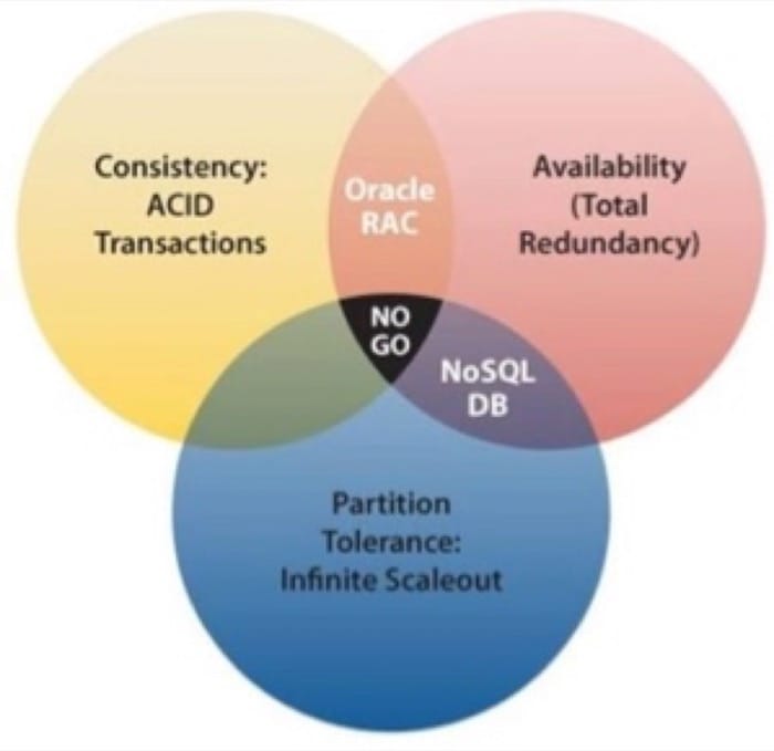
References

1. Eric Brewer (2000). "Towards Robust Distributed Systems." Proceedings of the Annual ACM Symposium on Principles of Distributed Computing.

Relational Databases

In the 1970s, Edgar F. Codd pioneered the relational database model, which shifted the focus away from the navigational approach to a data-centric approach. In the relational model, data is stored as fixed-length fields in normalized tables (Figure 4.17). In normalization, large tables can be divided into smaller and less redundant tables, and relationships can be defined between them. Codd went on to define various degrees of normalization for data stored in the relational model. In addition, the Structured Query Language (SQL) was developed at IBM to provide a reasonably intuitive language to create and manage databases.

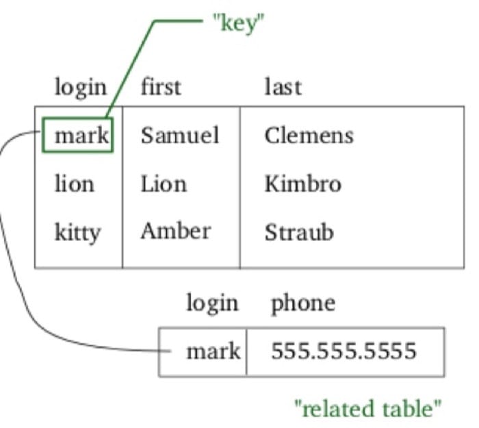
The concepts of relational databases were combined with SQL and used by IBM, which designed the System R and the DB2 relational database management systems (RDBMS), which were the precursors to all modern RDBMSs.

The typical features of modern RDBMSs include the following:

• Data is modeled as records in tables, and related records across tables are expressed as relations.
• Tables are defined by schemas, which impose rules on the types and valid inputs for each column (also known as a field) in a table.
• Tables are defined, accessed, and modified through a query language (typically SQL).

Modern RDBMSs provide application developers a complete data management solution that abstracts the notion of data management away from the application developer. Once a schema is designed, applications can store, retrieve, and modify records based on the rules specified in the schema. By specifying constraints on information in a database, applications can handle data in a more robust fashion, which is crucial to avoiding data inconsistencies in application programs. For example, a user database can validate the age of each user to be a non-negative integer between, say, 1 and 130. The database can then refuse to add a user whose age does not meet this constraint and can provide an automatic validation mechanism as the data is being stored.

Scaling in Traditional Databases

Traditional RDBMSs have been designed to run on a single machine, but as the amount of data or the number of concurrent users increase, the database must be scaled. Recall that databases can be scaled either vertically or horizontally.

Guaranteeing ACID properties across a distributed database where no single node is responsible for all data affecting a transaction presents additional complications. Network connections might fail, or one node might successfully complete its part of the transaction and then be required to roll back its changes because of a failure on another node. The need for distributed concurrency control mechanisms thus emerged.

An early example of distributed concurrency control was the two-phase commit (2PC) protocol. 2PC provides atomicity and consistency for distributed transactions to ensure that each participant in the transaction agrees on whether or not the transaction should be committed. In the first phase, one node (the coordinator) interrogates the other nodes (the participants) and sends a VOTE_REQUEST message to all participants (Figure 4.18). The participants then submit their vote on the transaction to the completed, either a VOTE_COMMIT or a VOTE_ABORT. In the second phase, the coordinator tallies the votes from every participant and issues a GLOBAL_COMMIT message if every participant voted in favor of the transaction or a GLOBAL_ABORT message if even one of the participants voted against the transactions (Figure 4.19). Finally, the participants commit the transaction or rollback based on the message received from the coordinator. The 2PC protocol thus guarantees strict consistency, as every transaction requires the global consensus among all nodes. Variants of 2PC include the three-phase commit (3PC) and the 2-phase locking protocol. However, these concurrency control protocols are expensive and affect performance at scale.

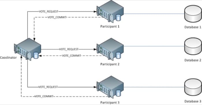
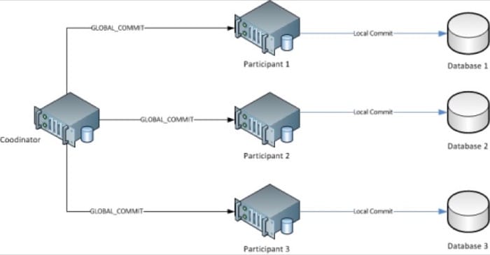
NoSQL Databases

Recall that Brewer’s CAP theorem proves that it is impossible to guarantee strict consistency and availability while being able to tolerate network partitions. This, in turn, led to various databases being designed with relaxed ACID guarantees, particularly in the case of consistency. An alternative to ACID is BASE (basically available, soft state, and eventual consistency).

• Basically available indicates that the system guarantees availability in terms of the CAP theorem. Small failures should not result in large disabilities of the system.
• Soft state indicates that the state of the system may change over time, even without input, because of the eventual consistency model.
• Eventual consistency means that given a sufficiently long period of time over which no changes are sent, all updates can be expected to propagate eventually through the system and the data will be consistent.

For example, assume a system with two transactions, A and B, running in parallel. Let A and B change the value of a variable x at the same time. Transaction A writes value a and transaction B writes the value b to variable x. Under a strict consistency model, the database will impose a total ordering of all transactions and guarantee that every read of the variable x will return its latest value. Under eventual consistency, the value of the variable x may not propagate to each and every node before the next read. Even after transaction B executes, some nodes may still see the variable x has value a. Since the system is eventually consistent, there is a possibility of conflicts emerging with regard to operations on the data. Conflicts can be resolved through mechanisms such as vector clocks or client-specified timestamps.

To understand why BASE is a useful model, consider the scenario of an e-commerce vendor that deals with millions of visitors every day. A bulk of the visitors are shopping around and browsing products. One of the elements that is on the screen is the available stock of a product. Now the vendor can calculate the available stock using an expensive transactional query that guarantees the value that is provided to the user at any given instant. However, this requires getting a consistent snapshot of the inventory database, which could in-turn lead to an expensive transaction, which is even more expensive if the vendor runs a distributed database. The vendor can only scale up so much until the performance of the query is poor. Instead, the vendor can use a lightweight query that returns a recent cached estimate of the number of available units of a particular product. Note here that the application can tolerate a stale or inaccurate values. The e-commerce website only cares if the customer decides to buy a particular product, during which it must use a transactional query to confirm the available inventory and update it after a customer completes a purchase.

Soft state and eventual consistency are techniques that work well in the presence of partitions and thus promote availability. A new class of databases emerged that follow BASE characteristics and have been dubbed as NoSQL databases. A few examples of NoSQL databases include Amazon’s Dynamo and Google’s BigTable. Eventual consistency can be tolerated as long as the application can tolerate stale data. Applications such as instant messaging, for example, are usually tolerant of the eventual consistency limitations.

The typical characteristics of NoSQL databases include

• No strict schema requirements
• No strict adherence to ACID properties for transactions
• Consistency traded in favor of availability

The tradeoff with NoSQL databases is between ACID properties (most notably consistency) and performance and scalability.

Types of NoSQL Databases

A limited taxonomy of NoSQL databases is illustrated in Figure 4.20.

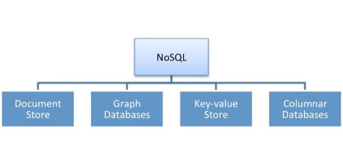
Document Stores

In contrast to RDBMSs, where data is stored as records with fixed-length fields, document stores store a document in some standard format or encoding. These DBs because popular because they can store a variety of data and their schema can change with time. The encoding may be in XML or JSON, as well as any arbitrary binary format such as PDFs or Office documents. These are typically called binary large objects (BLOBs). A document is addressed using a key, which can be indexed for fast retrieval. Clearly, document stores can be used to store and index documents or individual media in a manner than can be indexed using metadata. This allows document stores to outperform traditional file systems in searching and indexing capabilities. Examples of document stores include MongoDB and CouchDB.

Graph Databases

In graph databases, graph structures such as vertices and edges are used to represent and store data. Graph databases can be used to store data that has network-like properties between elements (e.g., a social network graph). Graph databases are a powerful tool for graph-like queries, for example, where you might want to find the shortest path between two elements. Figure 4.21 illustrates an example of a graph database with a vertex representing a person or a club and the edges representing membership or familiarity. Alice and Bob are represented using vertices with an edge that signifies the “knows” relationship connecting them. From this, we can see that Alice and Bob know each other. The relationship is further quantified using the “since” tag, which specifies that Alice has known Bob since 2001/10/03 and Bob has known Alice since 2001/10/04. Likewise, a group entity called “Chess” is defined with relationships indicated by edges to both Alice and Bob, which signifies that they are both members of a chess group.

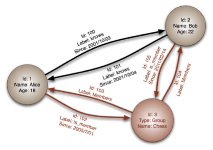
Queries in graph databases typically consist of graph traversals. For example, graphs can be used to compute the degrees of separation between two or more people in a social graph. Graph databases thus are great at representing networked information, with the relationship between entities occupying a key aspect of the representation. Examples of graph database software include Neo4j and VertexDB.

Key-Value Stores

Key-value (KV) store is a database model that maps keys to (possibly) more complex values. This type of database has the most amount of flexibility because keys can be mapped to arbitrary values or structures such as lists. The key-value pair constitutes an individual record in this model, and the keys are typically stored as a hash table. Hash lookups are fast and can be distributed easily, and for this reason, key-value stores can be scaled horizontally. Key-value stores typically support no more than the regular CRUD (create, read, update and delete) operations and may not natively support more advanced operations such as aggregations (e.g., averaging the values across key-value pairs) and joins (e.g., combining multiple-key value pairs into another key-value pair). Key-value stores are great for storing semi-structured information that is difficult to encapsulate within a rigid schema. The key-value relationship thus enables fast retrieval of data through an indexed key. Examples of key-value stores include Amazon DynamoDB and Apache Cassandra.

Columnar Databases

Columnar databases are a hybrid of RDBMSs and KV stores. Like relational databases, they store values in groups of zero or more columns, and as in key-value stores, values are queried by matching keys. However, in columnar databases, data is physically transposed and stored in column order instead of in row-order as in traditional RDBMSs. Operations such as modification of a subset of columns or aggregation of a column across all rows become more efficient, as entire rows do not have to be read to obtain the value of a single column. Furthermore, addition of columns to an existing table is inexpensive compared to traditional RDBMSs. Columnar databases have been traditionally developed with horizontal scalability as a primary design goal. As such, they are particularly suited to “big data” problems, living in clusters of tens, hundreds, or thousands of nodes. They also tend to have built-in support for features such as compression and versioning. Examples of columnar databases include HBASE and Vertica.

Comparing Popular Databases

The following table illustrates the differences between various popular databases that belong to each category.

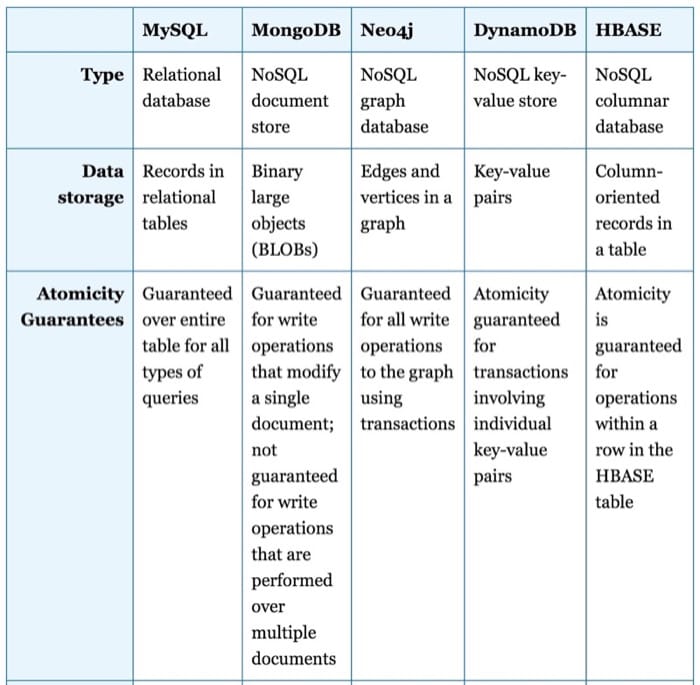
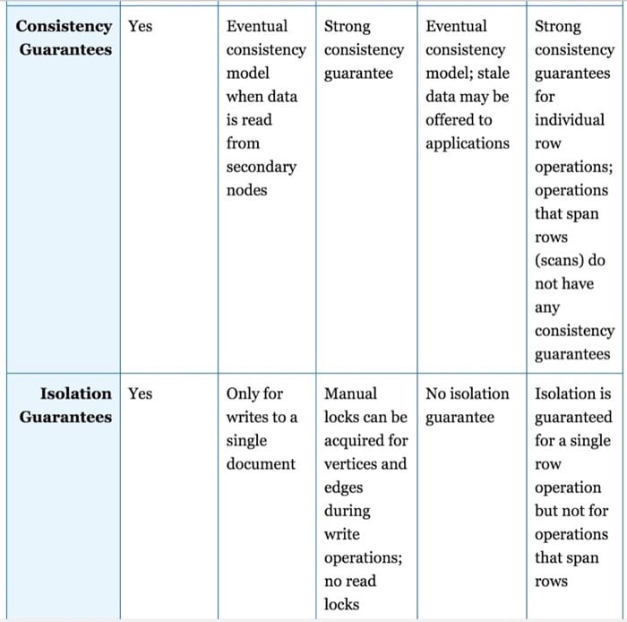
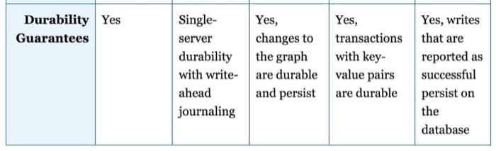
Following are some of the advantages of NoSQL databases.

• Data flexibility: NoSQL databases are designed with non-relational models and hence typically do not enforce a rigid schema. Document stores allow arbitrary information to be stored in some form of encoding (XML/JSON, etc.) or even in binary. Graph databases do not have schemas but a set of properties that are used in different kinds of edges or nodes. In key-value stores, for example, the value associated to a key can be a single value or a larger, more complex data structure such as a hash or list. In columnar stores, it is fast and easy to alter a table to add more columns if required.
• Scalability: Several NoSQL systems employ a distributed architecture from the ground up, unlike RDBMSs whose fundamental designs have not changed in decades. This means that NoSQL systems are built for high scalability. For example, Yahoo! has deployed a 1000+ node HBASE cluster with 1 PB of data, and such large data stores are not uncommon with companies such as Google, Amazon, and Facebook.
• Performance: By relaxing some of the ACID guarantees, NoSQL systems can take advantage of parallel access to data and provide faster performance than their traditional SQL counterparts.

Disadvantages of NoSQL databases include the following.

• Application developers can no longer rely on ACID guarantees and have to design for lack of consistency guarantees. They must account for the possibility of stale data from the database during reads or writes that are not fully committed to disk before the operation.
• NoSQL has lock-in because of a lack of standards. Even if data formats may be standardized through XML or JSON, each NoSQL product may have its own query/response formats. By comparison, moving between RDBMSs is easier because the data formats and query languages are largely standardized.

NewSQL Databases

NoSQL databases have been quite successful in very specific domains. The most popular avenue for NoSQL systems is the storage of big data for web-scale companies whose applications that can tolerate reduced consistency guarantees. However, this approach pushes some of the storage challenges to the application developer. As an example, the non-relational data model means that develops may have to implement their own joins if they ever need to combine data from two tables. They also have to handle eventually consistent data and ensure that their applications do not face any correctness issues with the lack of transactions. However, not all applications can give up these strong transactional semantics. There is a demand for database systems that can combine the best of both the relational and NoSQL worlds; these systems work using a relational model and SQL, with ACID transactions, while offering scalable performance that is similar to NoSQL systems.

NewSQL databases refer to the next generation of relational DBMSs that can scale like a NoSQL system, without fully giving up on SQL or some level of ACID properties for transactions. This can be done using multiple techniques, the most popular of which we will discuss here:

1. Shared-Nothing Architectures: A common design pattern in NewSQL systems is the adoption of a shared-nothing architecture. This is a system in which each node is completely independent (sometimes down to the level of individual threads), thus ensuring that there is no single point of contention across the system. This enables systems to have a high performance at scale because there is no need for expensive locking protocols.
2. In-Memory Systems: Another avenue for improving performance in database systems is to reduce the number of trips made to disk for a given query. An extreme version of this philosophy is to operate an entire database from memory, so that the database never has to go to disk.

H-Store and VoltDB

H-Store is a good example of a NewSQL system. H-Store is deployed on a cluster of nodes, using a shared-nothing architecture. At the heart of H-Store is a highly optimized single-threaded database engine which quickly processes individual queries. The database is then sharded across the cluster such that every individual core is responsible for a disjoint subset of the data. The data in h-store is stored in the memory of each of the nodes in the system.

Because each engine has exclusive access to all of the data at a partition, only one transaction at a time is able to access the data stored in the partition, eliminating the need for locks and latches in the system. As a result, no transaction will stall waiting for another transaction once started, at least for queries that do not span a single partition.

H-Store has its limitations. First, the lack of durable storage (as H-Store stores all data in-memory), coupled with the shared nothing architecture means that node failures can cause loss of data.

While H-Store was an academic project, the commercial realization of H-Store emerged as VoltDB. VoltDB has been improving and adding features to H-Store in order to address the shortcomings of VoltDB, including a logging mode to enchance the durability of the storage system.

Object Storage as a Cloud Service

We will now look at a special class of storage systems that are designed as a cloud service that is provided over the internet. In the context of our discussion on cloud storage thus far, object storage in clouds can be considered to be a special case of key-value stores provided as a service over the Internet.

Providing storage as a service to clients over the Internet requires abstracting the underlying storage implementation details and providing a simple and clean interface that can be used in applications. Cloud adopters are increasingly choosing the cloud object model for storage on the cloud.

With the concept of objects, object-based storage systems abstract the existing file system approach at a higher level. Object-based storage systems are typically layered over existing file systems. There is no notion of hierarchies in object-based storage systems, which instead use a flat data environment.

An object can be considered as a generic container that can store any arbitrary type of information. Designing interfaces for such arbitrary data may be difficult, but in storage parlance, a basic set of operations can be easily defined for any arbitrary object. These operations are create, read, update, and delete (CRUD), which are typically made available through some kind of API that can be accessed through HTTP or other network protocols using REST- or SOAP-style calls.

REST

Representational state transfer (REST) relies on a stateless, client-server, cacheable communications protocol and is typically implemented over HTTP. A stateless protocol treats each request as an independent operation, and each communication between a client and server is treated as an independent pair of requests and responses. Video 4.10 discusses HTTP and RESTful interfaces

Video 4.10: HTTP and RESTful Interfaces

REST is an architectural style for designing networked applications and does not refer to a single protocol. REST is a design strategy for communications among various entities in a networked application. The idea is to use a simple mechanism instead of CORBA, WSDL, or RPC to connect and transfer information between machines over a network. Any interface that uses REST principles is called a RESTful interface.

A RESTful interface uses HTTP requests to post (create and/or update), read (make queries and get information), and delete data. Thus, a RESTful interface can be used for CRUD operations.

A RESTful interface consists of the following components:

• A uniform resource identifier (URI), such as an HTTP URL through which the service can be accessed.
• An Internet media type for the data supported by the service (typically XML or JSON).
• A set of operations that is supported by the Web service using HTTP methods (GET, PUT, POST, and DELETE).
• An HTTP-driven API.

Thus, a program that needs to connect to a service with a RESTful interface can use standard HTTP GET, PUT, POST, and DELETE requests. An example of a REST request is covered shortly.

The major advantages of REST are that it is

• A platform-independent approach that is ideally suited for the Internet.
• A language-independent interface because all instructions are passed over HTTP so that, for example, a C# client can talk to a Python server.
• A standards-based communication because it runs on top of HTTP.
• Operational in the presence of firewalls as long as HTTP or HTTPS traffic is not filtered.

Object Storage Systems - Amazon S3

Video 4.11 covers the basics ideas behind Object Storage Systems:

Video 4.11: Object Storage Systems

An example of object-based storage on the cloud is Amazon’s Simple Storage Service (S3). S3 allows users to store objects in buckets. Each object can be created, read, and deleted. Note that in the S3 model, although no native update-object method exists, an entire object can be deleted and re-created, similar to a file overwrite. However, S3 supports object versioning and can maintain multiple versions of an object on S3 if it is explicitly enabled by the object owner.

Here is an example of a RESTful HTTP call to Amazon S3 to create a bucket named mybucket. The HTTP call includes authorization information for the client to access the bucket.

PUT /mybucket HTTP/1.1
Content-Length: 0
User/Agent: jClientUpload
Host: s3.amazonaws.com
Date: Sun, 05 Aug 2007 15:33:59 GMT
Authorization: AWS 15B4D3461F177624206A:YFhSWKDg3qDnGbV7JCnkfdz/IHY= LE:k3nL7gH3+PadhTEVn5EXAMPLE

S3 can process the request and will send back an HTTP response similar to the following:

HTTP/1.1 200 OK
x-amz-id-2: tILPE8NBqoQ2Xn9BaddGf/YlLCSiwrKP+OQOpbi5zazMQ3pC56KQgGk
x-amz-request-id: 676918167DFF7F8C
Date: Sun, 05 Aug 2007 15:30:28 GMT
Location: /mybucket
Content-Length: 0
Server: AmazonS3

In the response, Amazon has acknowledged the request, indicated that the request was successful (with a "200 OK" message), and returned some information regarding the request. The x-amz-id-2 and x-amz-request-id fields are unique identifiers that can be used to keep track of responses for troubleshooting and debugging purposes.

Cloud Object Storage Standards: CDMI

The lack of a common standard for object storage is an issue plaguing cloud object storage. The most popular cloud-based object storage system is Amazon S3, which is proprietary.

The Storage Network Industry Association (SNIA) is promoting an open standard for cloud objects, called cloud data management interface (CDMI).

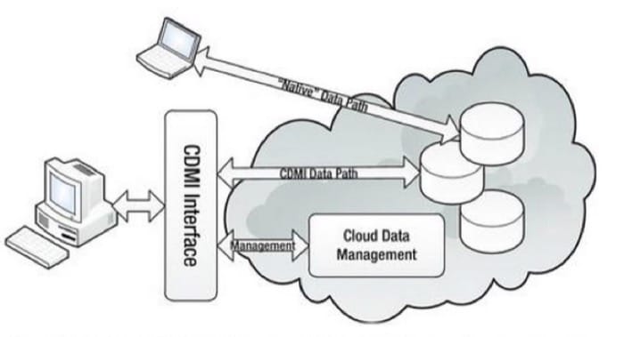
CDMI defines data objects and data containers with tagged metadata (as key-value pairs) and uses RESTful interfaces, with JSON as the data exchange format. CDMI can be used for accessing and managing data on a storage cloud (Figure 4.22). An example of a client interaction with a storage cloud using CDMI is shown in Figure 4.23.

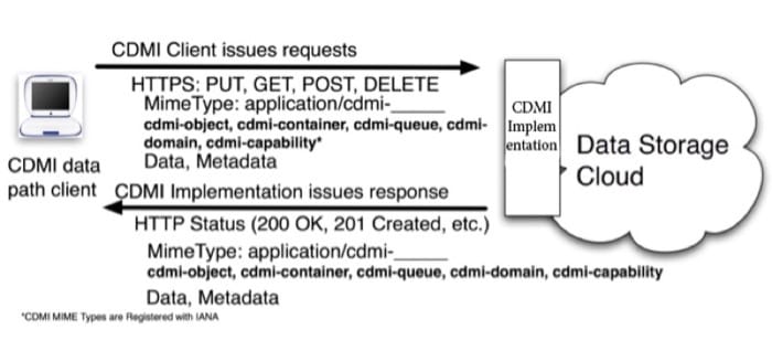
The CDMI client can issue requests over HTTPS, and the MimeType indicates the type of CDMI resource with which the client is interacting (an object, a container) and returns standard HTTP status codes, indicating the status of the request.

The CDMI model is illustrated in Figure 4.24. A CDMI resource exists on a root location, indicated by the root URI: https://. The example contains two containers, A and B, that contain one object each. Note that each CDMI entity can support metadata, as indicated with the key-value tags associated with every entity.

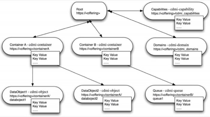
In addition, CDMI supports the following resource types:

• cdmi-capability: A special entity that describes the capabilities of this particular cloud store. This entity is important and can be used to discover the capabilities of a cloud (e.g., backup and replication).
• cdmi-domain: Allows for the creation of domains (e.g., groups of users with object access permissions).
• cdmi-queues: Allow for the creation of queues of objects that operate in first in, first out (FIFO) order. Applications can use such queues to implement notification or messaging systems.

The advantages of CDMI include the following:

• Its vendor-neutral specification of a cloud object storage system allows for simpler data migration from one cloud to another.
• It enables cloud peering for storage, which is a concept wherein resources from different clouds can be connected to enable seamless data sharing between clouds.
• It adheres to existing standards, such as RESTful interface for data access, and can work with multiple underlying storage abstractions, such as shared and networked file systems.
• It is a mature standard, which has a reference implementation and ISO standardization.

The disadvantage of CDMI is that its adoption is yet to be seen. The CDMI standard is backed by many storage companies, but it is not yet officially supported by vendors such as Amazon, and the standard's success remains unclear.

Summary

• Data can be characterized by its structure, dynamicity, and volume. It usually can be fixed or structured, static or dynamic.
• Storage technologies have been evolving to keep pace with ever-growing needs to store vast amounts of data.
• Different applications can exhibit different requirements in terms of capacity, performance, fault-tolerance, durability and others. Storage systems are designed to address these requirements in an efficient manner.
• Storage abstractions can be in the form of blocks on a block device, files on a file system, or as entities in a database.
• There are many types of file systems, such as local, shared, and networked file systems.
• Local file systems manage data on block devices (physical disks or LUNs). They map files to regions of the disk called blocks. File systems are designed with performance and dependability concerns in mind.
• A single file system can be expanded over multiple disks, typically using LVM/RAID.
• It is typical for storage to be consolidated in enterprise environments to facilitate pooling, sharing, and improving manageability of storage resources. Consolidated storage systems are typically shared among multiple servers using a storage area network (SAN).
• A distributed file system is a network file system with files distributed among multiple file servers. A file is stored whole on one of the file system servers that is part of the DFS.
• Distributed file systems have many design considerations, including fault tolerance, replication, consistency, and file-sharing semantics.
• Databases evolved from the navigational model to the modern relational database model and further to the NoSQL and NewSQL models.
• There are multiple design considerations for database systems.
• When the data is amenable to structuring, it is typical to organize it using a well-defined model (also known as a schema). Semi-strctured or unstructured data are typically stored in schema-less systems such as key-value stores.
• The CAP theorem states that any distributed storage system with shared data can have at most two of three desirable properties among the following: consistency, availability, and/or partition tolerance.
• An RDBMS models data into interconnected tables. A schema defines the rules on the types and valid inputs for each column of a table. Tables are defined, accessed, and modified through a query language (typically SQL).
• An RDBMS supports transactions by providing atomicity, consistency, isolation, and durability (ACID) guarantees.
• Traditional databases can be scaled either vertically or horizontally.
• Vertical scaling simply requires the underlying hardware (CPU, memory, disk, etc.) to be upgraded.
• With horizontal scaling, a database is distributed across multiple machines, either through replication (same data is stored across multiple machines) or sharding (data is distributed across multiple machines).
• Achieving ACID properties in a distributed database is challenging. Typically, a two-phase commit protocol (2PC) is used to ensure ACID properties in such databases. However, this approach affects performance at very large scales.
• NoSQL databases take a relaxed approach to strict consistency guarantees in order to provide availability and partition tolerance at large scale and high performance.
• A few types of NoSQL databases include document stores, graph databases, key-value stores, and columnar databases.
• NoSQL databases typically offer data flexibility, scalability, and high performance for large volumes of data when compared to traditional RDBMSs.
• Applications must take into account the relaxed consistency model of NoSQL data stores. Lack of standardization makes it difficult to migrate data from one database to another.
• NewSQL databases attempt to combine the relational data model and SQL interface of RDBMSes with the scalability and performance of NoSQL systems. This is done by reengineering the database engines to perform well at scale through in-memory storage and a shared-nothing architecture.
• Object stores provide an abstraction of an object (which is a generic container to store any arbitrary type of information) and a set of very basic operations—create, read, update, and delete (CRUD)—to enable online storage. They can be considered to be a service-oriented version of key-value stores.
• Object stores are typically accessed using an API that is accessed over the network using REST/SOAP-style calls.
• Amazon S3 is an example of an object store, and CDMI is an upcoming open standard that defines a cloud storage environment.