云计算 阅读材料 6 Cloud Software Deployment Considerations

Now that you have seen how a cloud data center runs, you may feel that all of the complexity is handled by the Cloud Service Providers (CSPs), and it is trivial to build a cloud application. However, to truly fulfil the promise of the cloud, developers must design and deploy their applications following a few best practices.

---

In this module, we look at how applications are to be deployed on the cloud to ensure fault tolerance and achieve high performance. The global presence of cloud data centers simplifies the process of reaching many end users, but deployment patterns must support easy scaling and fault-tolerance.

A cloud application must be economical, reachable with low-latency, support a large number of simultaneous users (high throughput), without any service degradation (fault tolerance and elasticity). Despite the tools that CSPs provide, building such an application requires a lot of planning.

In the last module of Unit 2, we will look at some common patterns around load balancing and scaling, as well as how robust applications should be built.

Last, we explore some additional challenges faced by responsive, interactive applications that use a large cluster of cloud computing resources and look at some solutions.

Programming the Cloud

Cloud Programming Considerations

Designing programs that are destined for the cloud requires special considerations. Depending on the type of application and the expected load, developers can utilize some of the features provided by cloud providers to enhance the scalability and maintainability of programs. Use of automatic scaling systems and load balancers allow developers to dynamically grow or shrink infrastructure based on the utilization of hardware or a program-computed load factor.

There are multiple considerations that a developer must account for when developing or migrating an application to the cloud, particularly those that concern performance and security.

Factors that Impact Application Performance on the Cloud

The environment in a cloud-centric data center is different from what developers might be used to when designing and deploying applications on owned infrastructure. Some developers find it hard to fine-tune or enhance the performance of their applications because they do not have access to the physical hardware layout or specifications on public clouds. We will try to enumerate some of the top concerns, with specific emphasis on factors that affect application performance on the cloud:

Resource Bandwidth and Latency

A primary concern for developing and deploying cloud applications is latency. Developers must plan their applications with strict latency requirements in mind. One approach is to compile the distribution of client locations. This will allow developers to find the optimal set of data center locations which can be used to optimize end-user performance and responsiveness. This is particularly true in web applications, where individual HTTP requests for static web content can represent an important fraction of the web page load times.

Apart from latency, applications may also have strict bandwidth requirements, particularly with those that deal with rich multimedia content such as audio and video. Many cloud providers allow cloud developers to specify performance parameters during provisioning in the form of IOPS requirements for compute and storage resources. In addition, many cloud providers allow developers to set up virtual networks. The implementation and adoption of Software Defined Networking and Storage (covered in future modules) provide additional insights into newer techniques used by data centers to manage traffic from multiple clients, while managing individual requirements as specified in the client SLOs.

The techniques mentioned above are primarily targeted for static content. A far more difficult problem is to optimize the latency of access to distributed data storage systems, particularly those that have to handle writes and updates. We will learn a bit more of these concerns in future modules.

Multi-tenancy

Applications on public data centers typically run on shared infrastructure. This aspect of cloud services raised several important issues. While modern virtualization technologies provide an isolated environment in terms of application environment and security, they typically cannot ensure performance isolation. Therefore virtualized resources on clouds cannot guarantee consistent performance at all times, the performance of a resource at any given time is a function of the total load on the resources from all tenants, also known as the interference experienced from other tenants sharing the same hardware.

Some cloud providers such as AWS provide clients the ability to provision certain types of resources (such as EC2 instances) on dedicated hardware. This provides protection against wide fluctuations in resource performance, delivering fairly consistent performance for the resources. However, dedicated hardware instances cost considerably more than regular on-demand instances, as AWS needs to assign a server exclusively for your resources.

A related aspect of multi-tenancy is the issue of provisioning variation, wherein identical requests for virtual resources on public clouds are not mapped identically onto physical resources, thereby causing a variation in performance [1] . For example, two identical requests for virtual machines (VM1 and VM2) could be routed to two different physical machines (A and B). Physical machine A might have four other tenants competing for resources on the same machine, while machine B may have only two. However, the client is charged the same for virtual machines VM1 and VM2, but can potentially experience different performance on these machines.

Security Settings

Public clouds are subject to increased attack vectors, as we saw in Unit 1. Developers must be extremely cautious in ensuring that they follow best practices, protocols and procedures when deploying and maintaining applications on the cloud. As a result, additional performance overheads may be experienced due to the use of security protocols mandated by public clouds.

Since we have already discussed these protocols in a previous module, we will not discuss it in detail again. Any code deployed on a public cloud should go through a strict process of manual and automated source code reviews and static analysis, as well as dynamic vulnerability analysis and penetration testing. Guidelines for deploying applications securely are shown on the next page.

References

1. Rehman, M.S and Sakr, M.F (2010). "Initial Findings for Provisioning Variation in Cloud Computing." 2010 IEEE Second International Conference on Cloud Computing Technology and Science (CloudCom).

Deploying Applications on the Cloud

Once a cloud application has been designed and developed, it can be moved to the deployment phase for release to clients. Deployment can be a multi-stage process, each involving a series of checks to ensure that the goals of the application are met.

Before deploying a cloud application into production, it is useful to have a checklist to assist in evaluating your application against a list of essential and recommended best practices. Examples include the deployment checklist from AWS and Azure. Many cloud providers provide a comprehensive list of tools and services that assist in deployment, such as this document from AWS.

The Deployment Process

The deployment of a cloud application is an iterative process which starts from the end of development right through to the release of the application on the production resources (Figure 2.28):

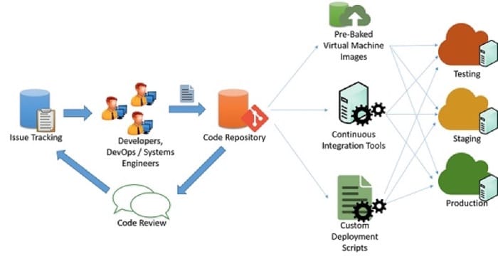
It is typical for cloud developers to maintain multiple concurrently running versions of their applications to pipeline deployment of their application to into various stages:

1. Testing
2. Staging
3. Production

Each of the three stages mentioned above should ideally have identical resources and configuration which allows developers to test and deploy the application and minimize the chances of inconsistencies stemming from a change in the environment and configuration.

Pipelining Application Changes

In a typical agile application development scenario (illustrated in the figure above), applications are maintained by a set of engineers and developers who work on issues and bugs using some kind of issue tracking mechanism. The changes to the code are maintained through a code repository system (say, svn, mercurial or git), where separate branches are maintained for release of code. After passing through code changes, reviews and approvals, the code can be pipelined into the testing, staging and production phases. This can be done in multiple ways:

Custom Scripts: Developers can use custom scripts to pull the latest version of the code and run specific commands to build the application and bring it into production state.

Pre-Baked Virtual Machine Images: Developers can also provision and configure a virtual machine with all the required environment and software to deploy their application. Once configured, the virtual machine can be snapshotted and exported to a virtual machine image (such as an AMI in AWS), and this image can be provided to various cloud orchestration systems to be automatically deployed and configured for a production deployment.

Continuous Integration Systems: In order to simplify the various tasks that are involved in deployment, Continuous integration (CI) tools can be used to automate tasks (such as retrieval of the latest version from a repository, building application binaries and running test cases) that need to be completed in the various machines that make up the production infrastructure. Examples of popular CI tools include: Jenkins, Bamboo, Travis. AWS Code Pipeline is an AWS-specific CI tool designed to work with AWS deployments.

Managing Downtime

Certain changes to the application may require partial or full termination of the application services to incorporate a change in the application back-end. Developers have to typically schedule a specific time of day to minimize interruptions to customers of the application. Applications that are designed for continuous integration may be able to perform these changes live on production systems with minimal or no interruption to the application’s clients.

Redundancy and Fault Tolerance

Best practices in application deployment typically assume that cloud infrastructure is ephemeral and may be unavailable or change at any moment. For example, virtual machines deployed in an IaaS service may be scheduled for termination at the cloud provider’s discretion, depending on the type of SLA.

Applications must refrain from hard-coding or assuming static endpoints for various components, such as databases and storage endpoints. Well designed applications should ideally use service APIs to query and discover resources and connect to them in a dynamic fashion.

Catastrophic failures in resources or connectivity can happen at a moment's’ notice. Critical applications must be designed in anticipation of such failures and must be designed for failover redundancy.

Many cloud providers design their data centers into regions and zones. A region is a specific geographic site which houses a complete data center, while zones are individual sections within a data center which are isolated for fault tolerance. For example two or more zones inside a data center may have separate power, cooling and connectivity infrastructure so that a fault in one zone will not affect the infrastructure in the other. Region and Zone information is typically made available by cloud service providers to clients and developers to design and develop applications that can utilize this isolation property.

Developers can therefore configure their application to use resources in multiple regions or zones in order to improve the availability of their application and tolerate failures that may happen across a zone or region. They will need to configure systems that can route and balance traffic across regions and zones. DNS servers can also be configured to reply to domain lookup requests to particular IP addresses in each zone, depending on where the request originated. This provides a method of load balancing based on the geographic proximity of clients.

Security and Hardening in Production

Running Internet applications on a public cloud must be done with care. Since cloud IP ranges are well-known locations for high-value targets, it is important to ensure that all applications deployed on the cloud follow best practices when it comes to securing and hardening endpoints and interfaces. Some very basic principles that should be followed include:

1. All software should be switched to production mode. Most software supports “debug-mode” for local testing and “production-mode” for actual deployments. Debug-mode applications generally leak a large deal of information to attackers who send it malformed inputs and hence provide an easy source of reconnaissance for hackers. No matter if you are using a web-framework like Django and Rails or a database like Oracle, it is important to follow the relevant guidelines for deploying production applications.
2. Access to nonpublic services should be restricted to certain internal IP addresses for admin access. Make sure that administrators cannot directly log in to a critical resource from the Internet without visiting an internal launchpad. Configure firewalls with IP address and port-based rules to allow the minimal set of required accesses, especially over SSH and other remote connectivity tools.
3. Follow the principle of least privilege. Run all services as the least privileged user that can perform the required role. Restrict the use root credentials to specific manual logins by system administrators who need to debug or configure some critical problems in the system. This also applies to access to databases and administrative panels. Accesses should generally be protected using a long, random public-private key pair, and this key pair should be stored securely in a restricted and encrypted location. All passwords should have strict strength requirements.
4. Use well-known defensive techniques and tools for intrusion detection and prevention systems (IDS/IPS), security information and event management (SIEM), application layer firewalls, and anti-malware systems.
5. Set up a patching schedule that coincides with patch releases by the vendor of the systems that you use. Often, vendors like Microsoft have a fixed release cycle for patches.

Build Fault-tolerant Cloud Services

Failures and Fault Tolerance

A large part of data center and cloud service management involves designing and maintaining a reliable service based on unreliable parts. The slide below (Figure 2.29) is a part of Google’s training for new hires, and should provide an idea of the large number (and types) of failures that are experienced regularly at a large data center.

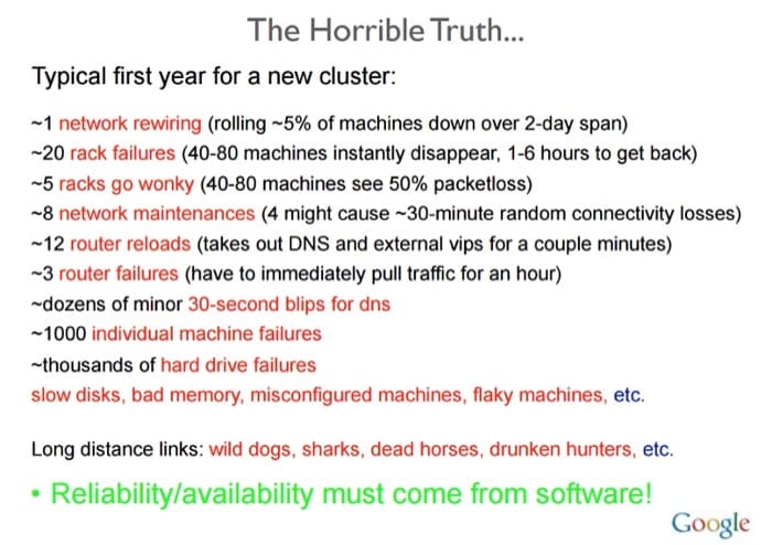
A failure in a system occurs as a result of an invalid state introduced within the system due to a fault. Systems typically develop faults of one of the following types:

1. Transient faults– Temporary fault in the system that corrects itself with time.
2. Permanent faults – Faults that cannot be recovered from and generally require replacement of resources.
3. Intermittent faults – Faults that occur periodically in a system.

Faults may affect the availability of the system by bringing down the services or performance of the system functionalities. A fault-tolerant system has the ability to perform its function even in the presence of failures in the system. On the cloud, a fault-tolerant system is often thought of as one that provides services in a consistent manner with lower downtime than the agreed Service Level Agreements (SLAs) allow.

Why is it Important?

Failures in large mission critical systems can result in significant monetary losses to all parties concerned. By the very nature of cloud computing systems having a layered architecture, a fault in one layer of the cloud resources can trigger a failure in other layers above, or hide access to the layers below.

For example a fault in any hardware component of the system can affect normal execution of a Software as a Service application running on a virtual machine using the faulty resources. Faults in a system at any layer have a direct relation to the Service Level Agreements between the providers at each level.

Proactive Measures

Service providers take several measures in order to design the system in a specific way to avoid known issues, or predictable failures.

Profiling and Testing

Load and stress testing cloud resources in order to understand possible causes of failure is essential to ensure the availability of services. Profiling these metrics helps in designing a system that can successfully bear the expected load without any unpredictable behavior.

Over-provisioning

This is the practice of deploying resources in volumes that are larger than the general projected utilisation of the resource at a given time. In situations where the exact needs of the system cannot necessarily be predicted, over-provisioning resources can be an acceptable strategy in order to handle unexpected spikes in loads.

Consider as an example an e-commerce platform that has average consistent load on their servers year round, but during the holiday season the expectation is that the load pattern will spike up rapidly. At these peak times, it is advisable to provision extra resources based on the historical data for peak usage. A rapid rise in traffic is typically difficult to accommodate in a short period of time. As discussed in later sections, there is a time cost associated with scaling dynamically which involves the time consuming steps of detecting a change in the load pattern and provisioning extra resources to accommodate the new load, which will require time. This time delay in adjustment can be enough to overwhelm and at worst crash the system or at best degrade the Quality of Service.

Over-provisioning is also a tactic used to defend against DoS (Denial of Service) or DDoS (Distributed DoS) attacks, which is when attackers generate requests designed to overwhelm a system by throwing large volumes of traffic at them as an attempt to make the system fail. In any attack, it always takes some time for the system detect and take corrective measures. While such analysis of request patterns is being made, the system is already under attack and needs to be able to accommodate the increased traffic until a mitigation strategy can be implemented.

Replication

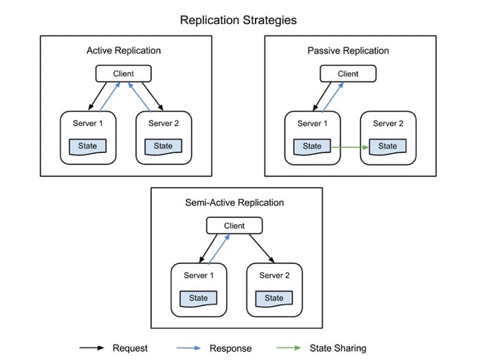
Critical systems components can be duplicated by using additional hardware and software components to silently handle failures in parts of the system without the entire system failing. Replication has two basic strategies:

• Active Replication, where all replicated resources are alive concurrently and respond to and process all requests. This means that for any client request, all resources receive the same request, all resources respond to the same request, and ensure that that the order of the requests is maintained to maintain state across all resources.
• Passive Replication, where only the primary unit processes requests and secondary units merely maintain state and take over once the primary unit fails. The client is only in contact with the primary resource, which relays the state change to all secondary resources. The disadvantage of passive replication is that there may be either dropped requests or degraded QoS when switching from the primary to the secondary instance.

There is also a hybrid strategy that is used, called semi-active, which is very similar to the active strategy with the difference that only the output of the primary resource is exposed to the client. The outputs of the secondary resources are suppressed and logged, and are ready to switch over as soon as a failure of the primary resource occurs. Figure 2.30 illustrates the differences between the replication strategies.

An important factor to consider in replication is the number secondary resources to use. Although this differs from application to application based on the criticality of the system- there are 3 formal levels of replication:

• N+1 - This basically means that for an application that needs N nodes to function properly, one extra resource is provisioned as a fail-safe.
• 2N - At this level one extra node for each node required for normal function is provisioned as fail-safe.
• 2N+1 - At this level one extra node for each node required for normal function and one additional node overall is provisioned as a fail-safe.

Reactive Measures

In addition to predictive measures, systems can take reactive measures and deal with failures as and when they happen:

Checking and Monitoring

All resources are constantly monitored in order to check for unpredictable behavior or loss of resources. Based on the monitoring information, recovery or reconfiguration strategies are designed in order to restart resources or bring up new resources. Monitoring can help in the identification of faults in the systems. Faults that cause a service to be unavailable are called crash faults and those that induce an irregular/incorrect behavior in the system are called byzantine faults.

There are several monitoring tactics that are used to check crash faults within a system. Two of them are:

1. Ping-Echo, where the monitoring service asks each resource for its state and is given a time window to respond
2. Heartbeat, where each instance sends status to the monitoring service at regular intervals, without any trigger.

Monitoring byzantine faults usually depends on the properties of the service being provided. Monitoring systems can check basic metrics like latency, CPU utilization, memory utilization, etc, and check against the expected values to see if the Quality of Service is being degraded. In addition application specific supervision logs are usually kept at each important service execution point and analysed periodically to see that the service is functioning properly at all times or whether there are injected failures in the system.

Checkpoint and Restart Several programming models in the cloud implement checkpoint strategies, whereby state is saved at several stages of execution in order to enable recovery to a last saved checkpoint. In data analytics applications, there are often long running parallel distributed tasks that run on Terabytes of data sets to extract information. Since these tasks are executed in several small execution chunks, each step in the execution of the program can save the overall state of execution as a checkpoint. At points of failures where individual nodes are unable to complete their work, the execution can be restarted from a previous checkpoint. The biggest challenge while identifying valid checkpoints to roll back to is when parallel processes are sharing information. A failure in one of the processes may cause a cascading rollback in another process, as the checkpoints made in that process can be a result of fault in the data shared by the failing process. You will learn more about fault tolerance for programming models in future modules.

Case Studies in Resiliency Testing

Cloud services need to be built with redundancy and fault-tolerance in mind, as no single component of a large distributed system can guarantee 100% availability or uptime.

All failures including failures of dependencies in the same node, rack, data-center or regionally redundant deployments need to be handled gracefully without affecting the entirety of the system. Testing the ability of the system to handle catastrophic failures is important as sometimes even a few seconds of downtime or service degradation can cause hundreds of thousands, if not millions of dollars in revenue loss.

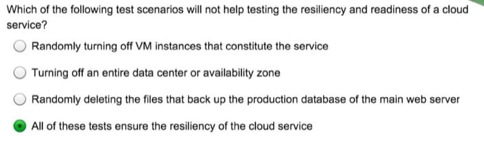
Testing for failures with real traffic needs to be done regularly so that the system is hardened and can cope when an unplanned outage occurs. There are various systems built to test resiliency, one such testing suite is Simian Army built by Netflix.

Simian Army consists of services (Monkeys) in the cloud for generating various kinds of failures, detecting abnormal conditions, and testing ability to survive them. The goal is to keep the cloud safe, secure, and highly available. Some of the Monkeys found in the Simian Army are:

1. Chaos Monkey: A tool that randomly picks a production instance and disables it to make sure the cloud survives common types of failure without any customer impact. Netflix describes Chaos Monkey as "The idea of unleashing a wild monkey with a weapon in your data center (or cloud region) to randomly shoot down instances and chew through cables -- all the while we continue serving our customers without interruption". This kind of testing with detailed monitoring can expose various forms of weaknesses in the system and automatic recovery strategies can be built based on the results.
2. Latency Monkey: A service that induces delays in between RESTful communication of different clients and servers, simulating service degradation and downtime.
3. Doctor Monkey: A service that finds instances that are exhibiting unhealthy behaviors (eg: CPU load) and removes them from service. It allows the service owners some time to figure out the reason for the problem and eventually terminates the instance.
4. Chaos Gorilla: A service that can simulate the loss of an entire AWS availability zone. This is used to test that the services automatically rebalance the functionality among the remaining zones without user-visible impact or manual intervention.

Load Balancing

The need for load balancing in computing stems from two basic requirements, a system employs replication to provide high availability and improves performance through parallel processing. High availability is the property of a service that is available for near 100% of the time when any client tries to access the service. The Quality of Service of a particular service generally includes several considerations such as throughput, latency requirements among others.

What is Load Balancing?

The most well-known form of load balancing is “Round robin DNS” employed by many large web services to load balance requests among a number of servers. Specifically, multiple front-end web servers, each with a unique IP address share a DNS name. To balance the number of requests on each of these web servers, large companies like Google maintain and curate a pool of IP addresses associated with a single DNS entry. When a client makes a request (for e.g. to the domain www.google.com), Google’s DNS would select one of the available addresses from the pool and sends it to the client. The simplest strategy employed to dispatch IP addresses is to use a simple round-robin queue, where after each DNS response, the list of addresses are permuted.

Before the advent of the cloud, DNS load balancing was a simple way to tackle the latency of long-distance connections. The dispatcher at the DNS server was programmed to respond with the IP address of the server that was geographically nearest to the client. The simplest schemes to do this tried to respond with the IP address from the pool that was numerically the closest to the IP address of the client. This method, of course, was unreliable, as IP addresses are not distributed in a global hierarchy. Current techniques are more sophisticated and rely on a software mapping of IP addresses to locations based on physical maps of Internet Service Providers (ISPs). Since this is implemented as a costly software lookup, this method yields more accurate results, but is expensive to compute. However, the cost of a slow lookup is amortized since the DNS lookup occurs only when the first connection to a server is made by the client. All subsequent communications happen directly between the client and the server that owns the dispatched IP address. An example of a DNS load balancing scheme is shown in the figure below.

The downside of this method is in the case of a server failure, the switch over to a different IP address is dependent on the configuration of the Time-To-Live(TTL) of the DNS cache. DNS entries are known to be long-living and updates are known to take over a week to propagate over the Internet. Hence, it is difficult to quickly “hide” a server failure from the client. This can be improved by reducing the validity (TTL) of an IP address in the cache, but this occurs at the cost of performance and increasing the number of lookups.

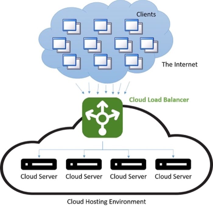
Modern load balancing often refers to the use a dedicated instance (or a pair of instances) that directs incoming traffic to the backend servers. For each incoming request on a specified port, the load balancer redirects the traffic to one of the backend servers based on a distribution strategy. In doing so the load balancer maintains the request metadata including information like Application protocol headers (such as HTTP headers). In this situation, there is no problem of stale information as every request passes through the load balancer.

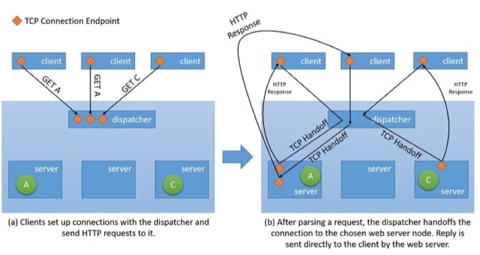
Though all types of network load balancers will simply forward the user’s information along with any context to the backend servers, when it comes to serving the response back to the client they may employ one of two basic strategies [1] :

1. Proxying - In this approach the load balancer receives the response from the backend and relays it back to the client. The load balancer behaves as a standard web proxy and is involved in both halves of a network transaction, namely forwarding the request to the client and sending back the response.
2. TCP Handoff - In this approach the TCP connection with the client is handed off to the backend server and therefore the server sends the response directly to the client, without going through the load balancer.

How Does This Help With Availability and Performance?

Load balancing is an important strategy to mask failures in a system. As long as the client of the system is exposed to a single endpoint that is balancing load across several resources, failures in individual resources can be masked from the client by simply servicing the request via a different resource. However it is important to note that the now the Load Balancer is the single point of failure of the service because if it fails for any reason, even if all backend servers are still functioning, no client request will be able to be served. Hence in order to achieve high availability, load balancers are often implemented in pairs.

Load balancing allows a service to distribute workloads across several compute resources in the cloud. Having a single compute instance in the cloud has several limitations. We have discussed earlier the physical limitation on performance, where more resources are required for increasing workloads. By using load balancing, larger volume of workloads can be distributed across multiple resources such that each resource can fulfil its requests independently and in parallel, thereby improving the throughput of the application. This also improves average service times since there are more servers to serve the workload.

Checking and monitoring services are key in enabling the success of load balancing strategies. A load balancer needs to ensure that every request is fulfilled by ensuring each resource node is available, if not then traffic is not directed that specific node. Ping-echo monitoring is one of the most popular tactic in order to check the health of a specific resource node. In addition to health of a node, some load balancing strategies require additional information such as throughput, latency, CPU utilization, etc., in order to evaluate the most appropriate resource to direct traffic.

Load Balancers must often guarantee high availability. The simplest way to do this is to create multiple load balancing instances (each with a unique IP address) and link it to a single DNS address. Whenever a load balancer instance fails for any reason, it is replaced with a new one, and all traffic is passed on to the failover instance with a small performance impact. Simultaneously, a new load balancer instance can be configured to replace the failed one, and the DNS records should be immediately updated.

Strategies for Load Balancing

There are several load balancing strategies in the cloud:

Equitable Dispatching

This is a static approach to load balancing where a simple round-robin algorithm is used to divide the traffic between all nodes evenly and does not take into consideration the utilisation of any individual resource node in the system or the execution time of any request. This approach tries to keep every node in the system busy and is one of the simplest approaches to implement. An important drawback to this approach is that heavy client requests may aggregate and hit the same data centers, causing a few nodes to get overwhelmed while others remain underutilised. However, this requires a very specific load pattern and has low probability of occurring in practice on a large number of clients and servers with fairly uniform connection distribution and capacity. This strategy also makes it difficult to implement caching strategies on the data center that take into account considerations like spatial locality (where you prefetch and cache data near the data that was currently fetched), since the next request made by the same client may end up on a different server.

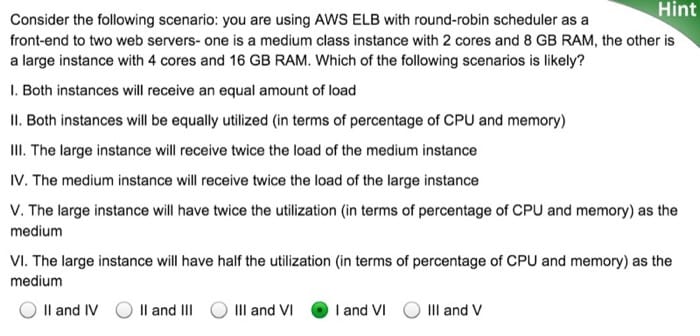
AWS uses this approach in their ELB (Elastic Load Balancer) offering. AWS ELB provisions load balancers that balance the traffic across the attached EC2 instances. Load balancers are essentially EC2 instances themselves with a service to specifically route traffic. As the resources behind the load balancer are scaled out, the IP addresses of the new resources are updated on the DNS record of the load balancer. This process takes several minutes to complete as it requires both monitoring and provisioning time. This period of scaling in the load balancer to be able to reach a point where it can handle a higher load is referred to as “warming up” the load balancer.

AWS’ ELB load balancers also monitor each resource attached for workload distribution in order to maintain a health check. A ping-echo mechanism is used to ensure all resources are healthy. ELB users can configure the parameters of the health check by specifying the delays and the number of retries.

AWS also supports “sticky sessions”, whereby metadata is added to maintain a shared context between the client’s browser and the load balancer so that all requests from that connection session are passed to the same backend server. This allows a web server to maintain session state transparently. Without sticky sessions, traditional web applications would struggle to function since a login that was completed on one of the web servers would not be valid if the user’s next request would be sent to a different web server.

Hash-based Distribution

This approach tries to ensure that at any point the requests made by a client through the same connection always ends up on the same server. In addition, in order to balance the traffic distribution of requests, it is done in a random order (it is important to note that this is different from round-robin). This has several advantages over the round-robin approach as it helps in session-aware applications where state persistence and caching strategies can be much simpler. It is also less susceptible to traffic patterns that would result in clogging on a single server since the distribution is random, but the risk still exists. In addition since every request needs to be evaluated for connection metadata in order to route to a relevant server, it introduce a small amount of latency to every request.

Azure Load Balancing Services uses such a hash-based distribution mechanism in order to distribute load. This mechanism creates a hash for every request based on – Source IP, Source Port, Destination IP, Destination Port and Protocol Type, in order to ensure that every packet from the same connection always ends up on the same server. The hash function is chosen such that the distribution of connections to servers is fairly random.

Azure provides health-checks via three types of probes - Guest Agent probe (on PaaS VMs), HTTP custom probes and TCP custom probes. All three probes provide health-check for the resource nodes via a ping-echo mechanism.

Other Popular Strategies

There are several other strategies used to balance load across multiple resources. Each of them uses different metrics to gauge the most appropriate resource node for a particular request:

1. Request execution time based strategies - These strategies use a priority scheduling algorithm, whereby request execution times are used in order to judge the most appropriate order of load distribution. The main challenge in using this approach is to predict the execution time of a particular request.
2. Resource utilization based strategies – These strategies use the CPU utilization on each resource node to balance the utilization across each node. The load balancers maintain an ordered list of resources based on their utilization and thus direct requests to the least loaded node.

Other Benefits of Employing a Load Balancer

Having a centralized load balancer lends itself to several strategies that can used to increase the performance of the service. However it is important to note that this strategy only works as long as the load balancer is not under insurmountable load, otherwise the load balancer itself becomes the bottleneck. Some of these are listed below:

• SSL Offload - Network transactions via SSL have a an extra cost associated with them since they need to have processing for encryption and authentication. Instead of serving all requests via SSL, the client connection to the load balancer can be made via SSL, while redirect requests to each individual server can be made via HTTP. This reduces the load on the servers considerably. Additionally security is maintained as long as the redirect requests are not made over an open network.
• TCP Buffering - This is a strategy to offload clients with slow connections on to the load balancer in order to relieve servers that are serving responses to these clients.
• Caching - In certain scenarios, the load balancer can maintain a cache for the most popular requests (or request that can be handled without going to the servers, like static content) so that it reduces the load on the servers.
• Traffic Shaping - For some applications a load balancer can be used to delay/reprioritize the flow of packets such that traffic can molded to suit the server configuration. This does affect the QoS for some requests, but makes sure that the incoming load can be served.

References

1. Aron, Mohit and Sanders, Darren and Druschel, Peter and Zwaenepoel, Willy (2000). "Scalable content-aware request distribution in cluster-based network servers." Proceedings of the 2000 Annual USENIX technical Conference.

Scaling Resources

One of the important advantages of the cloud is the ability scale resources into a system on-demand. Scaling up (provisioning larger resources) or scaling out (provisioning extra resources) can help in reducing the load on a single resources by decreasing utilization as a result of increased capacity or broader distribution of the workload.

Scaling can help in improving performance by increasing the throughput, since a larger number of requests can now be served. This also helps in improving latency since a reduced number of requests are queued during peak loads on a single resource. In addition this can also help in improving the reliability of the system by reducing the resource utilization to be farther away from the breaking point of the resource.

It is important to note that although the cloud enables us to easily provision newer or better resources, cost is always an opposing factor that needs to be considered. Therefore even though it is beneficial to scale up/out, it is also important to recognize when to scale in/down in order to save costs. In an n-tier application it is also essential to pinpoint where the bottlenecks are and which tier to scale, whether it is the data tier or server tier.

Scaling resources is facilitated by load balancing (we discussed this earlier), which helps in masking the scaling aspect of a system by hiding it behind a consistent endpoint.

Scaling Strategies

Horizontal Scaling (Scale Out/In)

Horizontal scaling is a strategy where additional resources can be added into the system or extraneous resources can be removed from the system. This type of scaling is beneficial for the server tier, when the load on the system is unpredictable and fluctuates inconsistently. The nature of the fluctuating load makes it essential to efficiently provision the correct amount of resources to handle the load at all times.

A few considerations that make this a challenging task is the spin up time of an instance, the pricing model of the cloud service provider and the potential loss in revenue from degrading Quality of Service by not scaling out in time. As an example let’s consider the following load pattern (Figure 2.33):

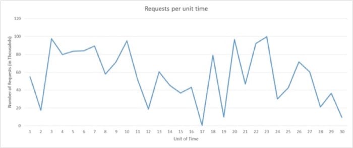
Let us imagine we are using Amazon’s Web Services, let us also imagine that each unit of time is equivalent to 3 hours of actual time and that we require one server to serve 5k requests. If you consider the load during the time units 16 to 22, there is an enormous fluctuation in the load. We can detect a fall in demand at right around time unit 16 and start to reduce the number of allocated resources. Since we are going from roughly 50k requests to almost 0 requests in the space of 3 hours, academically we can save the cost of 10 instances that would have been up at time 16.

Now let us imagine instead that each time unit is equal to 20 mins of actual time. In that case spinning down the all the resources at time unit 16 only to spin up new resources after 20 mins will actually increase the cost instead of saving, since AWS bills each compute instance on an hourly basis.

In addition to the above two considerations, a service provider will also need to evaluate the losses they will incur by providing degraded QoS during time unit 20, if they only have capacity for 90k requests instead of 100k requests.

The scaling depends on the characteristics of the traffic and its ensuing load generated at a web service. If the traffic follows a predictable pattern, for example based on human behavior such as streaming movies from a web service in the evening, then the scaling can be predictive in order to maintain the QoS. However, in many instances, the traffic cannot be predicted and the scaling systems need to be reactive based on different criteria as the examples above showed.

Vertical Scaling (Scale Up/Down)

There are certain kinds of loads for service providers that are more predictable than others. For example if you know from historical patterns that the number of requests will always be between 10k-15k, then you can comfortably assume that one server that can serve 20k requests will be good enough for the service provider’s purposes. These loads may increase in the future, but as long they increase in a consistent manner, the service can be moved to larger instance, that can serve more requests. This is suitable for small applications that experience a low amount of traffic.

The challenge in vertical scaling is that there is always some switch-over time that can be considered as down time. This is because in order to move all operations from the smaller instance to a larger instance, even if the switch-over time is mere minutes, the Quality of Service does degrade during that interval.

In addition, most cloud providers provide compute resources in increasing compute power by doubling the compute power of a resource. Therefore the granularity in scaling up is not as high as it is in horizontal scaling. So even if the load is predictable and steadily increasing as the popularity of the service increases, many service providers choose to do horizontal scaling instead of vertical scaling.

Considerations for Scaling

Monitoring

Monitoring is one of the most crucial element in scaling resources as it enables you to have metrics that can be used to interpret what parts of the system to scale and when to scale it. Monitoring enables analyzing traffic patterns or resource utilization in order to make an educated assessment to scale resources in order to maximize QoS along with profit.

There are several aspects of resources that are monitored in order to trigger scaling of resources. The most common metric is resource utilization. For example a monitoring service can track the CPU utilization of each resource node and scale resources if the usage is excessive or too low. If for instance the usage for each resource is higher than 95% then it is probably a good idea to add more resources since the system is under a heavy load. Service providers usually decide these trigger points by analyzing the breaking point of resource nodes, when they will start to fail, and mapping out their behavior under various levels of load. Though, for cost reasons, it is important to make maximum utilization out of each resource, it is advisable to leave some room for the Operating System to allow for overhead activities. Similarly if the utilization is significantly below say 50%, then it is possible that not all the resource nodes are required and can be un-provisioned.

In practice, service providers usually monitor a combination of several different metrics of a resource node to evaluate when to scale resources. Some of these include CPU utilization, Memory Consumptions, Throughput, Latency, etc. AWS provides CloudWatch as an additional service that can monitor any AWS resource and provide such metrics. There are other solutions available in the market as well like Nagios.

Statelessness

A stateless service design lends itself to a scalable architecture. A stateless service essentially means that the client request contains all the information necessary to serve a request by the server. The server does not store any client related information on the instance and does store any session related information on the server instance.

Having a stateless service helps in switching resources at will, without any configuration required to maintain the context (state) of the client connection for subsequent requests. If the service is stateful, then the scaling of resources needs to implement a strategy to transfer the context from the existing node configuration to the new node configuration. However there are techniques to implement stateful services like maintaining a network cache such as Memcached where the context is shared across the servers.

Deciding What to Scale

Depending on the nature of the service, different resources need to be scaled depending on the requirement. For the server tier, as the workloads increase, depending on the type of application, it may increase the resource contention for either CPU, memory, network bandwidth, or all of the above. Monitoring the traffic allows us to identify which resource is getting constrained and appropriately scale that specific resource. Cloud Service Providers do not necessarily provide scalability granularity to only scale compute or memory, but they do provide different types of compute instances that specifically cater to compute heavy or memory heavy loads. So for example for an application that has memory intensive workloads, it would be more advisable to scale up the resources to memory optimized instances, or for applications that need to serve a large number of requests that are not necessarily compute heavy or memory heavy, scaling out multiple standard compute instances might be a better strategy.

Increasing hardware resources may not always be the best solution for increasing the performance of a service. Increasing the efficiency of the algorithms used within the service can also help in reducing resource contention and improve utilization, removing the need to scale physical resources.

Scaling the Data Tier

In data-oriented applications, where there is a high number of reads and writes (or both) to a database or storage system, the round trip time for each request is often limited by the hard disk I/O read and write times. Larger instances allow for higher I/O performance for reads and writes which can improve seek times on the hard disk can in turn result in a large improvement in the latency of the service. Whereas having multiple data instances in the data tier can improve the reliability and availability of the application by providing failover redundancies. Replicating data across multiple instances has additional advantages in reducing network latency if the client is served by a data center physically closer to it. Sharding or partitioning of the data across multiple resources is another horizontal data scaling strategy where instead of simply replicating the data across multiple instances, data is partitioned into several partitions and stored across multiple data servers.

The additional challenge when it comes to scaling the data tier is that of maintaining all the three facets of Consistency (a read operation on all replicas is the same), Availability (reads and writes always succeed) and Partition Tolerance (guaranteed properties in the system are maintained when failures prevent communication across nodes) in the system. This is often referred to as the CAP theorem which in short states that within a distributed database system, it is very difficult to obtain all three properties completely and thus may at most exhibit a combination of two of the properties. You will learn more about database scaling strategies and the CAP theorem in future modules.

Dealing with Tail Latency

We have already discussed several optimization techniques used on the cloud to reduce latency. Some of the measures we studied include scaling resources horizontally or vertically and using a load balancer to route requests to the nearest available resources. This page delves more deeply into why, in a large data center or cloud application, it is important to minimize latency for all requests, and not just optimize the general case. We will study how even a few high-latency outliers can significantly degrade the observed performance of a large system. This page also covers various techniques to create services that provide predictable low-latency responses even if the individual components do not guarantee this. This is a problem that is especially significant for interactive applications where the desired latency for an interaction is below 100ms.

What is Tail Latency?

Most cloud applications are large, distributed systems often rely on parallelization as a source of reducing latency. A common technique is to fan-out a request received at a root node (for e.g. a front-end web server) to many leaf nodes (back-end compute servers). The performance improvement is driven both by the parallelism of the distributed computation, and also by the fact that extremely expensive data-moving costs are avoided. We simply move the computation to where the data is stored. Of course, each leaf node concurrently operates on hundreds or even thousands of parallel requests.

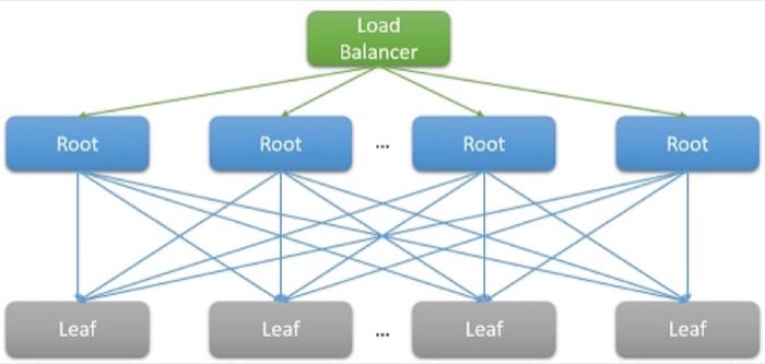
Consider the example of searching for a movie on Netflix. As a user begins to type in the search box, this will generate several parallel events from the root web server, which include at least the following requests:

1. to the autocomplete engine to actually predict the search being made based on past trends and the user’s profile,
2. to the correction engine which finds errors in the typed query based on a constantly adapting language model,
3. individual search results for each of the component words of a multi-word query, which must be combined together based on the rank and relevance of the movies,
4. additional post-processing and filtering of results to meet the user’s “safe-search” preferences

Such examples are extremely common. A single Facebook request is known to contact thousands of memcached servers, whereas a single Bing search often contacts over ten thousand index servers.

Clearly, the need for scale has led to a large fan-out at the back-end for each individual request serviced by the front-end. For services that are expected to be “responsive” to retain their user base, heuristics show that responses are expected within 100 ms. As the number of servers required to resolve a query increases, the overall time often depends on the worst performing response from a leaf node to a root node. Assuming that all leaf nodes must complete executing before a result can be returned, the overall latency must always be greater than the latency of the single slowest component.

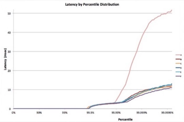
Like most stochastic processes, the response time of a single leaf node can be expressed as a distribution. Decades of experience have shown that in the general case, most (>99%) requests of a well-configured cloud system will execute extremely quickly. But often, there are very few outliers on a system that execute extremely slowly.

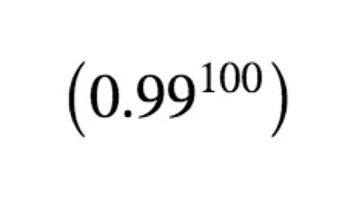
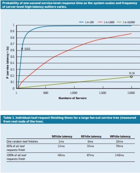
Consider a system where all leaf nodes have an average response time of 1 ms, but there is probability of a 1% that the response time is greater than 1000 ms (one second). If each query is handled by only a single leaf node, the probability of the query taking longer than one second is also 1%. However, as we increase the number of nodes to 100, the probability that the query will complete within one second drops to 36.6%, which means that there is a 63.4% chance that the query duration will be determined by the tail (lowest 1%) of the latency distribution.

If we simulate this for a variety of cases, we see that as the number of servers increase, the impact of a single slow query is more pronounced (notice that the graph below is monotonically increasing). Also, as the probability of these outliers decreases from 1% to 0.01%, the system is substantially lower.

Just like we designed our applications to be fault-tolerant to deal with resource reliability problems, it should be clear now why it is important for applications to be “tail-tolerant”. To be able to do this, we must understand the sources of these long performance variabilities and identify mitigations where possible and workarounds where not.

Variability in the Cloud: Sources and Mitigations

To resolve the response time variability that leads to this tail latency problem, we must understand the sources of performance variability [1] .

1. The use of shared resources: Many different VMs (and applications within those VMs) contend for a shared pool of compute resources and in rare cases it is possible that this contention leads to low-latency for some requests. For critical tasks, it may make sense to use dedicated instances and periodically run benchmarks when idle, to ensure that it behaves correctly.
2. Background daemons and maintenance: We have already spoken about the need for background processes to create checkpoints, backups, update logs, collect garbage and handle resource clean up. However, these can degrade the performance of the system while executing. To mitigate this, it is important to synchronize disruptions due to maintenance threads to minimize the impact on the flow of traffic. This will cause all variation to occur in a short, well-known window rather than randomly over the lifetime of the application.
3. Queueing: Another common source of variability is the burstiness of traffic arrival patterns [1] . This variability is exacerbated if the OS uses a scheduling algorithm other than FIFO. Linux systems often schedule threads out-of-order to optimize the overall throughput and maximize utilization of the server. However, studies have found that using FIFO scheduling in the OS reduces tail latency but may also reduce the overall throughput of the system.
4. All-to-all incast: The pattern shown in Fig 2.34 above is known as all-to-all communication. Since most network communication is over TCP, this leads to thousands of simultaneous requests and responses between the front-end web server and all the back-end processing nodes. This is an extremely bursty pattern of communication and often leads to a special kind of congestion failure known TCP incast collapse [1] [2] . The intense sudden response from thousands of servers leads to many packet drops and retransmissions, eventually causing a network avalanche of traffic for packets of data that are very small. Large data centers and cloud applications would often need to use custom network drivers to dynamically adjust the TCP receiving window and the retransmission timer. Routers may also be configured to drop traffic that exceeds a specific rate and reduce the size of the sending.
5. Power and temperature management: Finally, variability is a byproduct of other cost reduction techniques like using idle states or CPU frequency down-scaling. A processor may often spend a non-trivial amount of time scaling up from an idle state. Turning off such cost optimizations lead to higher energy usage and costs, but lower variability. This is less of a problem in the public cloud as pricing models rarely consider internal utilization metrics of customers’ resources.

Experiments conducted on AWS EC2 instances have found that the variability of such systems are much worse on the public cloud [3] , typically due to imperfect performance isolation of virtual resources and the shared processor. This is exacerbated if many latency-sensitive jobs are executed on the same physical node as CPU-intensive jobs.

Living with Variability: Engineering Solutions

Many of the sources of variability above have no fool-proof solution. Hence, instead of trying to resolve all of the sources that inflate the latency tail, cloud applications must be designed to be tail-tolerant. This, of course, is similar to the way that we design applications to be fault-tolerant since we cannot possibly hope to fix all possible faults. Some of the common techniques to deal with this variability are:

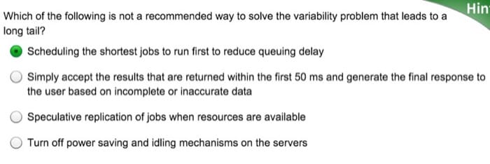
1. "Good enough" results: Often, when waiting to receive results from 1000s of nodes, the importance of any single result may be assumed to be quite low. Hence, many applications may choose to simply respond to the users with results that arrive within a particular, short latency window and discard the rest.
2. Canaries: Another alternative that is often used for rare code paths is to test a request on a small subset of leaf nodes in order to test if it causes a crash or failure that can impact the entire system. The full fan-out query is only generated if the canary does not cause a failure. This is akin to sending a canary (bird) into a coal mine to test if it is safe for humans.
3. Latency-induced probation and health checks: Of course, a bulk of the requests to a system are too common to test using a canary. Such requests are more likely to have a long-tail if one of the leaf nodes is performing poorly. To counter this, the system must periodically monitor the health and latency of each leaf node and not route requests to nodes that demonstrate low performance (due to maintenance or failures).
4. Differential QoS: Separate service classes can be created for interactive requests, allowing them to take priority in any queue. Latency-insensitive applications can tolerate longer waiting time for their operations.
5. Request Hedging: This is a simple solution to reduce the impact of variability by forwarding the same request to multiple replicas and using the response that arrives first. Of course, this can double or triple the amount of resources required. To reduce the number of hedged requests, the second request may only be sent if the first response has been pending for greater than the 95th-percentile of the expected latency for that request. This causes the extra load to be only about 5%, but reduces the latency tail significantly (in the typical case shown in Fig 2.35, where the 95th-percentile latency is much lower than the 99th-percentile latency).
6. Speculative execution and selective replication: Tasks on nodes that are particularly busy can be speculatively launched on other underutilized leaf nodes. This is especially effective if a failure in a particular node causes it to be particularly overloaded.
7. UX-based solutions: Finally, the delay can be intelligently hidden from the user by having a well designed user interface which reduces the sensation of delay experienced by a human user. Techniques to do this may include the use of animations, showing early results or engaging the user by sending relevant messages.

Using these techniques, it is possible to significantly improve the experience of the end-users of a cloud application to the peculiar problem of a long tail.

References

1. Li, J., Sharma, N. K., Ports, D. R., & Gribble, S. D. (2014). "Tales of the Tail: Hardware, OS, and Application-Level Sources of Tail Latency.." Proceedings of the ACM Symposium on Cloud Computing. ACM.
2. Wu, Haitao and Feng, Zhenqian and Guo, Chuanxiong and Zhang, Yongguang (2013). "ICTCP: Incast Congestion Control for TCP in Data-Center Networks." IEEE/ACM Transactions on Networking (TON). IEEE Press.
3. Xu, Yunjing and Musgrave, Zachary and Noble, Brian and Bailey, Michael (2013). "Bobtail: Avoiding Long Tails in the Cloud." 10th USENIX Conference on Networked Systems Design and Implementation. USENIX Association.
4. Dean, Jeffrey and Barroso, Luiz Andr{'e} (2013). "The tail at scale." Communications of the ACM. ACM.
5. Tene, Gil (2014). "Understanding Latency - Some Key Lessons and Tools." QCon London.

Economics for Cloud Applications

CSPs are taking great pains to attract users from their traditional deployments. Public IaaS cloud prices have been steadily and steeply falling ever since the launch of their services. On average, for most major CSPs, prices have fallen by 20-30% per year since 2013.

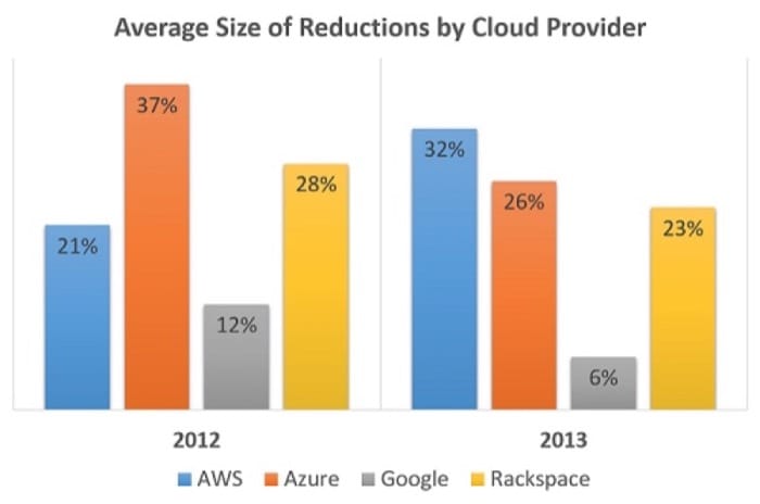
However, despite these decreasing prices, cloud adoption still must be done with care. To truly gain the cost benefits of the cloud, it is important to understand, budget, plan, monitor and carefully analyze your usage. Also, it is difficult to choose between CSPs for individual use cases, since there is no standard way for CSPs to package resources, nor do they always follow the same pricing models.

Pricing Models

Cloud providers generally charge for resources based on one of the following 3 types of parameters:

1. Time Based: Resources are charged based on the amount of time they are provisioned to the user. For example, you pay a certain amount per hour/day/month/year to have a virtual machine running on an IaaS cloud. The granularity of the charging period varies from cloud provider to cloud provider. Amazon, for example charges users per hour on a non-prorated basis.
2. Capacity Based: Users are charged based on the amount of a particular resource that is utilized or consumed. This is a popular charging model for cloud storage systems. For example, users are charged a certain amount for storing a gigabyte on cloud object storage systems such as S3 and Azure Blobs.
3. Performance Based: In many cloud providers, users can select a higher performance level for resources by paying a higher rate. For virtual machines, larger, more powerful machines with more CPU, Memory and Disk capacity can be provisioned at a higher hourly rate.

Based on these charging parameters, CSPs, such as AWS, use one of the following common pricing models:

1. On-demand / pay-as-you-go pricing: This is generally the most expensive pricing model for long-term usage. Payments are made for a very short period of usage (generally metered in minutes or hours). The advantages are that there is no need for a long-term contract, making it very flexible to scale in and out based on the current need. Although not common, it is possible for CSPs to increase costs during high demand and decrease it during low demand. This is a great model for service providers, as well as for cloud users who are just beginning to use the cloud.
2. Reserved instances / Subscription-based pricing: Instead of paying an hourly or per-minute rate, a user can choose to pre-pay and reserve a resource for a fairly long period of time (weeks or months). This often leads to significantly high markdowns (20-50%) but requires a long-term commitment. Within reserved pricing models, the payment schemes can vary from prepaid to contractually obliged periodic payments.
3. Spot pricing: Spot pricing is a way for CSPs to deal with excess unutilized capacity by offering it for sale at significantly lower prices than on-demand resources. For example,AWS often offers markdowns of 80-90% on spot EC2 resources. The prices are determined by a user auction, where users bid the maximum amount that they are willing to pay for a resource. The biggest downside is that the resources can often be terminated at any time if the spot price increases beyond the actual bid price. Spot resources are ideal for short-running, non-critical jobs that can be executed speculatively.

Generally reserved instances should be used to meet the base requirements of the system. If an application needs 2 instances 80% of the time, 3 instances 15% of the time and 4 instances 5% of the time, you would generally reserve 2 instances for the lifetime of the application and scale out either using on-demand or spot instances. As mentioned, on-demand instances should only be chosen while scaling out if the application is business critical or if the differential between the on-demand price and the current spot price is offset by the risk of sudden termination. This is often a business-case specific decision.

How to Optimize Cost Utilization

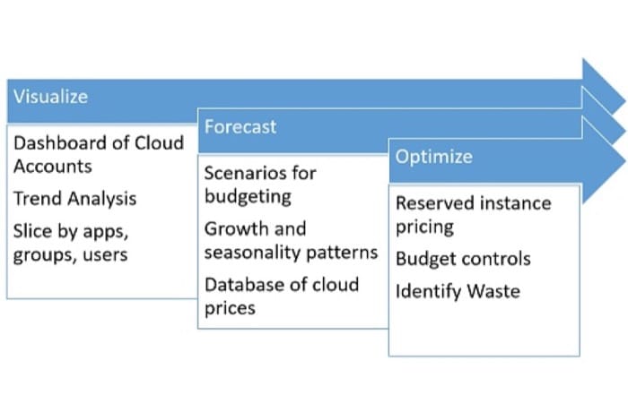
To use the cloud in a cost-effective manner, enterprises must develop a mature process for choosing the resources to deploy, monitor and visualize usage, as well as a clear mechanism to identify waste and optimize utilization.

Before considering cost requirements, an organization must plan the amount of work that it is capable of completing in a given period based on fixed resources like the amount of staff, while dealing with physical constraints like inventory management, overhead due to transportation, material handling etc. The provisioning of IT resources must be designed to meet or exceed the physical capacity of the organization. This is extremely important, because the elasticity provided by the cloud tempts development teams to simply add resources as needed, without considering the cost implications of their decisions.

The first step when attempting to reduce expenditure on the cloud is to match resource types with the actual requirement for the application. This may mean selecting between EC2 VMs with different memory configurations, or number of cores. There is no simple way to do this, apart from testing and benchmarking the application across different resource types.

Even if an application performs better on a more expensive resource class, it is important to verify if the performance improvement is proportional to the cost increase. For example, if there is a 1.2x improvement in an application using a VM that is 7.5x more expensive than the base, it might make more sense to horizontally scale out the base resource to improve the performance.

It is important to build a monitoring and visualization system to monitor the various resources being used. The monitoring system must be designed to trigger scaling events in response to observed patterns of overload or idleness. Often, infrastructure teams choose to scale up or out aggressively, while they scale down or in more conservatively. Though this approach is more expensive in terms of resource provisioning, it theoretically provides a higher Quality of Service than operating near peak capacity all of the time.

That being said, organizations often underestimate the need to scale down and terminate rarely used resources. When planning to run different components of an application, it is important to categorize the utilization into different bins, based on the approximate duration for which it will be used. For instance, any jobs that are run for a short time on a nightly or weekly basis should not use resources 24/7. Idle resources should also be flagged and terminated (based on certain rules) by the monitoring system.

An important technique that ties into cost optimization is that of tagging resources. Tagging is the process of assigning labels to resources that allow them to be identified by monitoring and analytics tools. Tagging also enables custom rules to be defined per-tag, including access control lists to resources, billing alerts and specific scaling policies. Commonly used tags specify the owner (user or group) of a particular resource, the environment to which it belongs (e.g. production, backup, staging, testing), the cost center in charge of paying the bill, etc. When analyzing expenditure, this enables the generation of grouped views based on particular applications, as well as on specific development or testing teams.

Case Study: Netflix's Ice System

As one of the largest AWS customers in the world, it is crucial for Netflix to have clear visibility about their expenditure. To support this requirement, they use an internally designed tool known as Ice. Ice relies on tags and resource metadata to build a dynamic dashboard that allows resources to be grouped by user, team, region, type, pricing model or any custom tag. It also supports the amortization of one time costs such as reserved instances over the lifetime of the resource. All of the data is periodically generated using AWS Billing APIs.

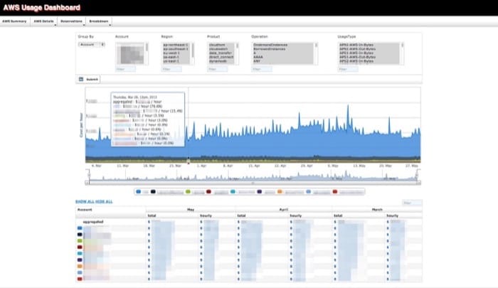
This tool has been released as a part of their Open Source initiative. Many companies (as well as CMU’s cloud computing course staff) use Ice or variants to gain insights into AWS usage and expenditure. It helps influence if any future resources should be reserved for the long-term (at cheaper prices), and identifies users or teams who overspend. All large cloud deployments should follow a similar process of planning & budgeting, monitoring & visualization, and forecasting & optimization.

Programming the Cloud Summary

• Cloud applications must take precautions to ensure that they use resources that help them meet their bandwidth and latency requirements, as well as follow security best practices.
• Applications deployed on the cloud are often subject to performance variance due to the shared nature of the cloud.
• The cloud makes it easy to maintain several different environments apart from production. Applicaton pipelines are maintained using code repository and version control systems and automated using Continuous Integration tools.
• Planning for failure is crucial. Redundancy is the key technique used to ensure resilience- often ensure using replicas deployed across availability zones and regions.
• Redundant resources are generally monitored and accessed using a central Highly Available load balancer. High Availability is ensure by switching over to a backup instance when one fails.
• Companies like Netflix and Facebook inject large random (or planned) failures in their data centers and cloud operations to test for fault tolerance.
• Load Balancing also supports horizontal scaling, whereby more identical resources can be thrown at a problem. The other type of scaling is vertical- where the size or capacity of existing resources is increased.
• Horizontal scaling across too many nodes leads to the problem of Tail Latency, where the performance of the application is determined by it's slowest component. This is both due to variability of performance on the cloud and also because applications with a large fan-out trigger bursts of activity at each stage.
• Finally, the lack of standardization and high competitiveness of the cloud market leads to interesting opportunties and challenges to minimize costs.